Outline
Focus: Improving staggered iteration between multiphase reaction transport and geomechanics
- Problems we were trying to solve
- Challenges we encountered
- Numerical algorithms
- Looking at poroelasticity as inspiration
- A new preconditioned staggered iteration
- Numerical experiments
- Problems we can now solve
Intro
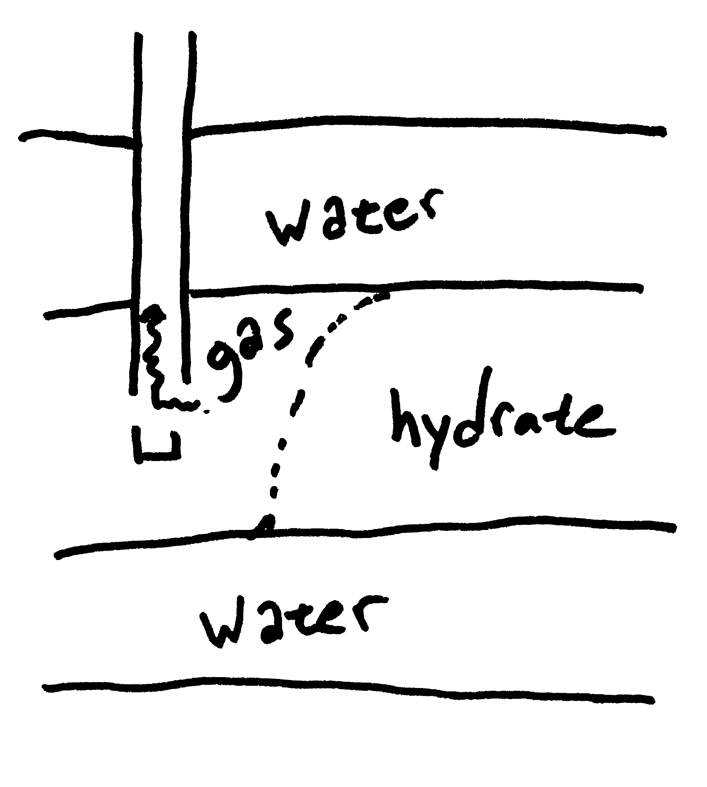
• Motivating problems are hydrate dissociation problems
• Wildly varying fluid compositions and mechanical properties
• Large changes causes drastic changes to the fluid mixture properties
• Properties vary greatly in space and time: can't estimate a priori
• Very soft sediments with soft gases and stiff liquids and ices
Challenges:
- Difficult to marry two physical descriptions
- One code for flow simulation, one code for geomechanics
- Slow convergence of staggered iteration
- Iteration can diverge when pore pressure dominates skeleton in stiffness
- Iteration can fail due to small valid ranges of in multiphase relations
What we have to work with:
- Ideally, one would develop a fully coupled simulator from the ground up
- That is easier said than done
- Disjoint development between multiphase chemistry and computational mechanics
- The problem is hard, not just writing the software
- Current boat is having two distinct solvers
- Working in TOUGH+ and Millstone
- Multiphase flow is very tricky: make mechanics package do the heavy-lifting
- Fortran calls C calls Python calls C calls Python-generated C
General System of Equations
Coupled transport, kinetics, and momentum balances:
Solve for $p,T,X$, and $u$ such that: \begin{eqnarray} \frac{\mathrm{d}m}{\mathrm{d}t} = & \nabla \cdot q + s & \} \text{balance of mass}\\ \frac{\mathrm{d}X}{\mathrm{d}t} = & r & \}\text{reactions (possibly equilibrium)} \\ 0 = & \nabla \cdot \sigma + f & \} \text{balance of momentum (quasistatic)} \end{eqnarray} Plus statemachine logic for phase change: \begin{eqnarray} state = \text{transition}(state; p,X,T) \end{eqnarray}
First: How We Solve It Now
Pick numerical methods that are best for each set of equations.
- Reaction-transport in reservoirs needs a very fine mesh
- Integral Finite Difference Method with TOUGH+ for reaction transport
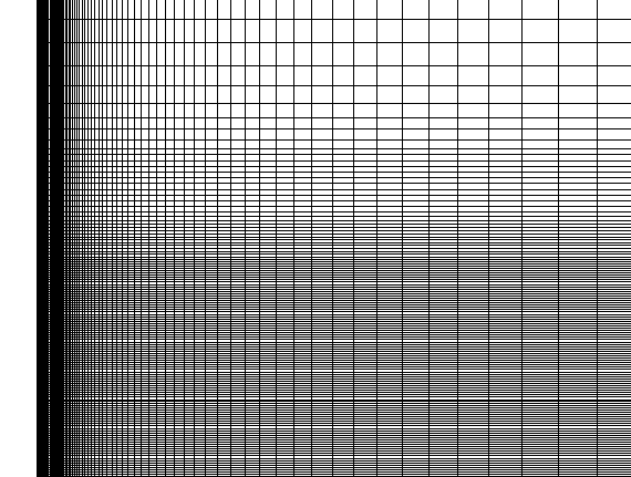
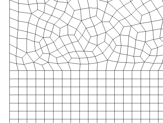
- Finite Element Method with Millstone for mechanics
- One-to-one aspect ratio problem for mechanics solved by using two meshes
- Axisymmetry in mechanics reduces unknowns and improves numerical performance
Problem fields are on two meshes
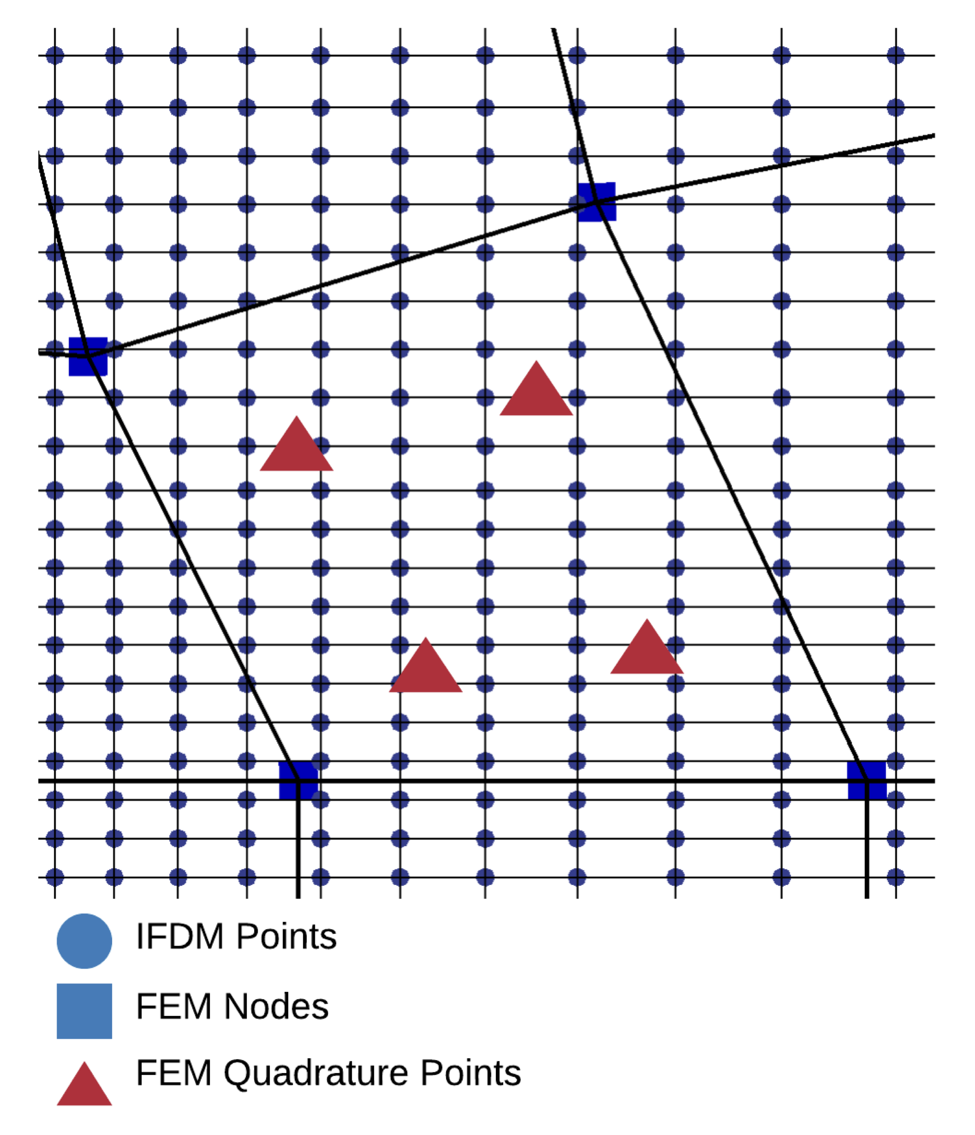
Have an additional interpolation step
Queiruga, Moridis, and Reagan, "Simulation of Gas Production from Multilayered Hydrate-Bearing Media with Fully Coupled Flow, Thermal, Chemical and Geomechanical Processes Using TOUGH+Millstone. Parts 1-3," Transport in Porous Media, 2019
Solving the Algebraic Equations
At each timestep, we're solving two nonlinear algebraic problems:
\begin{align} F(p,T,X,...)= & 0\left.\right\} \text{flow code}\\ M(u)= & 0\left.\right\} \text{mechanical code} \end{align}To really do Newton's method we would need: \begin{align} \left[\begin{array}{cc} \frac{\partial F}{\partial p} & \frac{\partial F}{\partial u}\\ \frac{\partial M}{\partial p} & \frac{\partial M}{\partial u} \end{array}\right]\left\{ \begin{array}{c} \Delta p^{k}\\ \Delta u^{k} \end{array}\right\} =-\left\{ \begin{array}{c} F^{k}\\ M^{k} \end{array}\right\} \end{align} E.g. in hydraulic fracturing the fluid pressure must be fully coupled like this or else it won't converge.
Hard to formulate those cross-terms:
- Very different discretizations on different meshes
- Two codes due to seperate development legacies
- Bigger matrix systems, harder to partition and solve in parallel
- Won't necessarily yield better performance
General Staggered Algorithm
For each Newton loop $k$ in the timestep:
- Solve mechanical stiffness using $K_d$ \begin{equation} \Delta u^{k+1} = [\mathtt{K}(K_d)] \,\,\backslash\,\, \{\mathtt{R(p^k,\sigma^k)} \} \end{equation}
- Increment Stress with $K_d$ \begin{equation} \Delta \sigma^{k+1} = \left(\left(K_d+\frac{2}{3}G\right) \nabla \cdot + 2G\nabla^s \right) : \Delta u^{k+1} + \alpha \mathbf{I} \Delta p^{k} \end{equation}
- Solve flow Jacobian with new volume \begin{equation} \Delta p^{k+1} = [\mathtt{J}(V^{k+1})]\,\,\backslash\,\,\{\mathtt{R}(V^{k+1})\} \end{equation}
- Do state transitions \begin{equation} state^{k+1} = \text{transition}(state^{k},p^{k+1}) \end{equation}
- Repeat until $\left|\Delta p\right|<\mathtt{tol\_flow}$ and $\left|\Delta u\right|< \mathtt{tol\_mech}$
General Algorithm
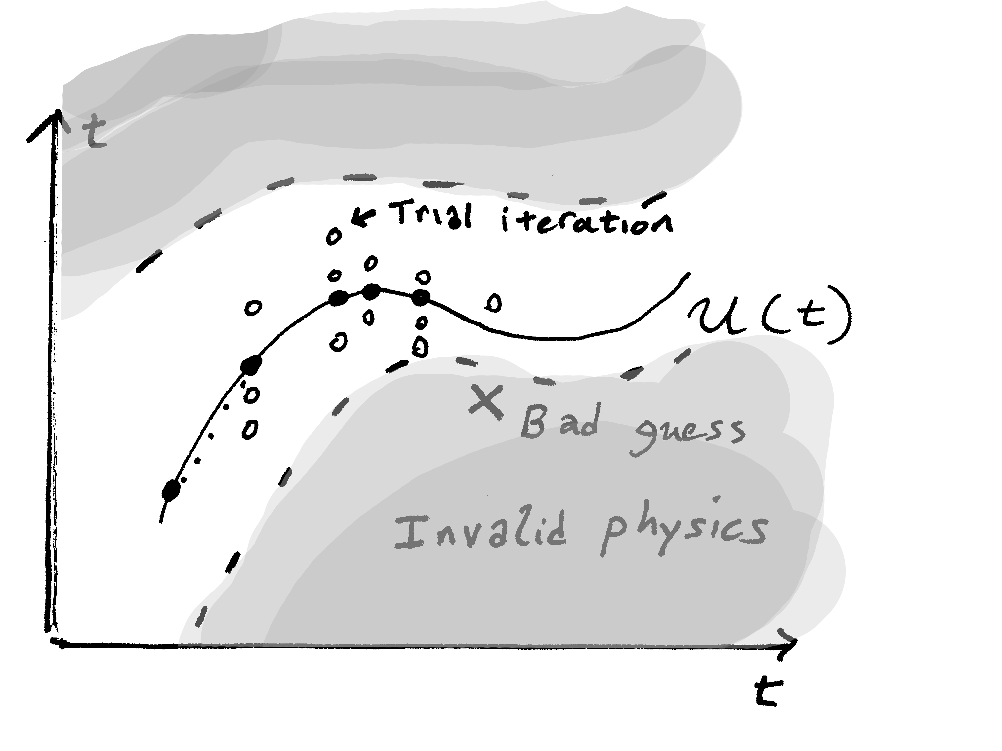
Staggering the two solvers is the same as this: \begin{equation} \left[\begin{array}{cc} \frac{\partial F}{\partial p} & 0\\ 0 & \frac{\partial M}{\partial u} \end{array}\right]\left\{ \begin{array}{c} \Delta p^{k}\\ \Delta u^{k} \end{array}\right\} =-\left\{ \begin{array}{c} F^{k}\\ M^{k} \end{array}\right\} \end{equation} Problematic when $\left| \frac{\partial M}{\partial p} \right| > \left| \frac{\partial M}{\partial u}\right|$: fluid stiffer than skeleton.
- Easy to implement.
- More iterations (no quadratic convergence!)
- Potentially a lot of over-shoot during the staggering.
- Exacerbates state transition logic.
This is catastrophic in large-range multiphase flow problems: \begin{equation} F(p_{bad}) = \text{raise out of range error} \end{equation} Physical descriptions have limits! May never be able to solve the system.
Can we find some matrix $C$ that helps? \begin{equation} \left[\begin{array}{cc} \frac{\partial F}{\partial p} & 0\\ 0 & \frac{\partial M}{\partial u}+C \end{array}\right]\left\{ \begin{array}{c} \Delta p^{k}\\ \Delta u^{k} \end{array}\right\} =-\left\{ \begin{array}{c} F^{k}\\ M^{k} \end{array}\right\} \end{equation}
Limited Range
Poroelasticity
The poroelastic constitutive response for the fluid pore pressure is \begin{equation} \mathrm{d}p=-M\alpha\nabla\cdot\mathrm{d}\mathbf{u}+M\nabla\cdot\left(\mathbf{q}\mathrm{d}t\right) \end{equation} where the poroelastic coefficient is \begin{equation} M^{-1} = \phi K_f^{-1} + (\alpha - \phi) K_s^{-1} \end{equation} where $\mathbf{q}\mathrm{d}t$ is an differential fluid volume into the control volume.
For the total stress, the constitutive response is, \begin{equation} \mathrm{d}\sigma=-\alpha\mathrm{d}p\mathbf{I}+\left(K_{d}-\frac{2}{3}G\right)\nabla\cdot\mathrm{d}\mathbf{u}\mathbf{I}+2G\nabla^{s}\mathrm{d}\mathbf{u}. \end{equation}
Note: We use the law for $\sigma$, but not $p$
Have nonlinearity in composition-dependent properties; e.g. in hydrate, $K$ and $G$ are function of saturation $S$: \begin{eqnarray*} K = K_{0}(1-S)+K_{1}S, \quad G = G_{0}(1-S)+G_{1}S \end{eqnarray*}
Reworking Poroelasticity
We can substitute $\mathrm{d}p$ for a familiar form: \begin{equation} \mathrm{d}\sigma=\left(K_{u}-\frac{2}{3}G\right)\nabla\cdot\mathrm{d}\mathbf{u}+2G\nabla^{s}\mathrm{d}\mathbf{u} + \alpha^2 M \nabla\cdot\left(\mathbf{q}\mathrm{d}t\right) \mathbf{I} \end{equation} where the undrained bulk modulus is: \begin{equation} K_{u} = K_d + \alpha^2 M \end{equation}
Making the analogy to our matrix system, we had (note: more variables than $p$) \begin{equation} \left[\begin{array}{cc} 1 & M\alpha\mathrm{tr}\\ \alpha\mathbf{I} & K_{d} \end{array}\right]\left\{ \begin{array}{c} \mathrm{d}p\\ \mathrm{d}u \end{array}\right\} =-\left\{ \begin{array}{c} f\\ m \end{array}\right\} \end{equation} and are trying to do: \begin{equation} \left[\begin{array}{cc} 1 & M\alpha\mathrm{tr}\\ 0 & K_{d}+\alpha^{2}M \end{array}\right]\left\{ \begin{array}{c} \mathrm{d}p\\ \mathrm{d}u \end{array}\right\} =-\left\{ \begin{array}{c} f\\ m - \alpha f \mathbf{I} \end{array}\right\} \end{equation} Triangularized the system so solving $\mathrm{d}u$ first would substitute into $\mathrm{d}p$ equation closer to the answer.
General Balance of Mass
Caveat: Poroelasticity only holds in the linear regime! (Small changes)
Actual balance of mass that the reservoir simulator solves is: \begin{equation} \frac{\partial}{\partial t} \rho = \nabla \cdot \mathbf{q} \end{equation} where we assumed: \begin{equation} \rho = \rho_0 ( 1+ p / K_f ) \end{equation} Flow simulators use very complicated nonanalytic formulations for $\rho$.
- $K_f$ and $M$ varies greatly especially at phase changes
- Don't necessarily have relations for $K_f$ for every possible scenario
- Varies spatially as well as temporally
Very complicated...
def gibbs_region1(T,p):
    p1_star = 1.653e7
    T1_star  = 1.386e3
    n1 = [ 0.14632971213167e00, -0.84548187169114e00,
          -3.7563603672040e+00,  3.3855169168385e+00,
          -0.95791963387872e00,  0.15772038513228e00,
          -1.6616417199501e-02,  8.1214629983568e-04,
           2.8319080123804e-04, -6.0706301565874e-04,
          -1.8990068218419e-02, -3.2529748770505e-02,
          -2.1841717175414e-02, -5.2838357969930e-05,
          -4.7184321073267e-04, -3.0001780793026e-04,
           4.7661393906987e-05, -4.4141845330846e-06,
          -7.2694996297594e-16, -3.1679644845054e-05,
          -2.8270797985312e-06, -8.5205128120103e-10,
          -2.2425281908000e-06, -6.5171222895601e-07,
          -1.4341729937924e-13, -4.0516996860117e-07,
          -1.2734301741641e-09, -1.7424871230634e-10,
          -6.8762131295531e-19,  1.4478307828521e-20,
           2.6335781662795e-23, -1.1947622640071e-23,
           1.8228094581404e-24, -9.3537087292458e-26]
    i1 = [ 0, 0,0, 0, 0, 0, 0, 0, 1,1, 1, 1,1, 1, 2, 2, 2, 2, 2, 3, 3, 3,
          4, 4,4, 5, 8,  8, 21, 23, 29, 30, 31, 32  ]
    j1 = [ -2, -1, 0, 1, 2, 3, 4, 5, -9, -7, -1, 0,1, 3, -3, 0, 1,3, 17, -4,
          0, 6, -5, -2, 10, -8, -11, -6, -29, -31, -38, -39, -40, -41  ]
    p_i = p/p1_star
    t_i = T1_star/T
    return R*T*sum([ n*(7.1-p_i)**I*(t_i-1.222)**J
            for n,I,J in zip(n1,i1,j1)])
density_region1,enthalpy_region1 = density_enthalpy(gibbs_region1)
Control Volume Simulations
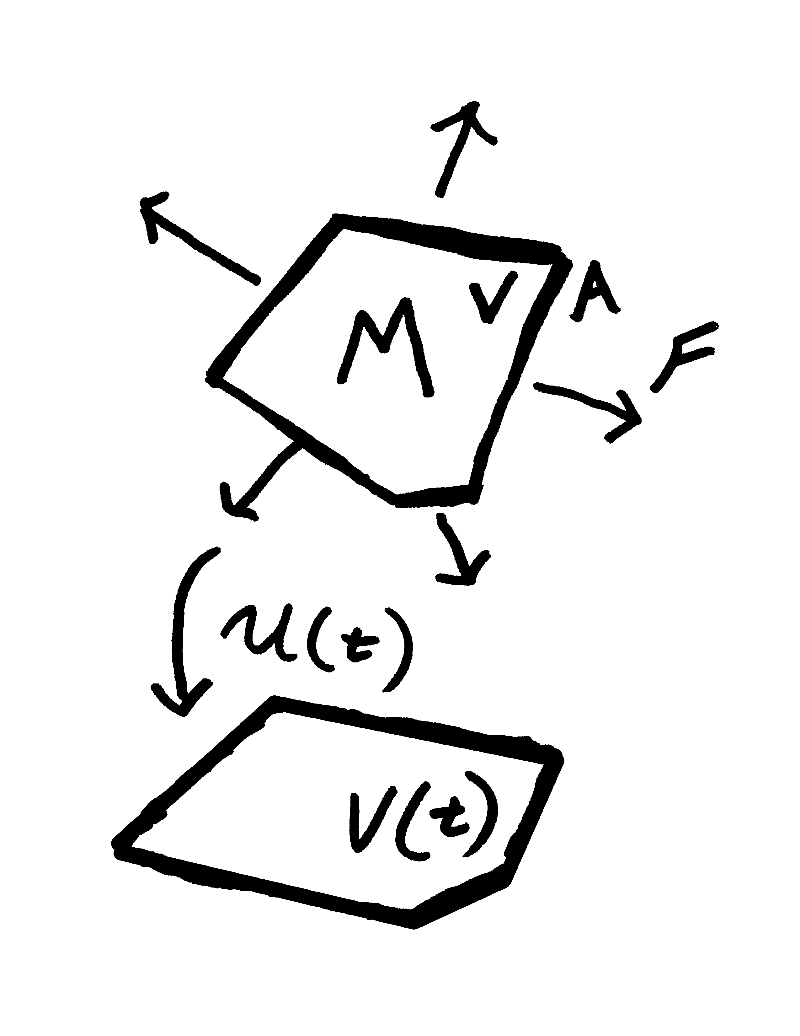
Solving balance with fluxes: \begin{equation} \frac{\mathrm{d}}{\mathrm{d}t}M_{comp}=\sum_{facets}F_{comp} \end{equation} Masses and fluxes are integrals over discrete domains and facets: \begin{equation} M_{comp}=\int_{\Omega}\phi\sum_{phase}S^{phase}\rho_{comp}^{phase}X_{comp}^{phase}\mathrm{d}^{3}x \end{equation} and: \begin{equation} F_{comp}=\int_{\Gamma}\sum_{phase}\mathbf{q}_{comp}^{phase}\cdot\mathbf{n}\mathrm{d}^{2}x \end{equation}
Flow and mechanics are coupled through volume of $\left|\Omega\right| = V(t)$ \begin{equation} \frac{\mathrm{d}V}{\mathrm{d}t} = V(t)\frac{\mathrm{d}}{\mathrm{d}t} \mathrm{tr} \varepsilon \end{equation} Poroelastic formulation uses the product rule to extract this term: \begin{equation} \frac{\mathrm{d}\rho V}{\mathrm{d}t}= V \frac{\partial \rho}{\partial p}\frac{\mathrm{d}p}{\mathrm{d}t} + \rho \frac{\mathrm{d}V}{\mathrm{d}t} \end{equation} (Derive from transformation of $\nabla_x\cdot$ to $\nabla_X\cdot$ given $x(t)=X+u(t)$)
Slightly Improved Staggered Algorithm
For each Newton loop $k$ in the timestep:
- Solve mechanical stiffness using $K_u^*$ \begin{equation} \Delta u^{k+1} = [\mathtt{K}(K_d+\alpha^2 M)] \,\,\backslash\,\, \{\mathtt{R(p^k,\sigma^k)} \} \end{equation}
- Increment Stress with $K_d$ \begin{equation} \Delta \sigma^{k+1} = \left(\left(K_d+\frac{2}{3}G\right) \nabla \cdot + 2G\nabla^s \right) : \Delta u^{k+1} + \alpha \mathbf{I} \Delta p^{k} \end{equation}
- Solve flow Jacobian with new volume \begin{equation} \Delta p^{k+1} = [\mathtt{J}(V^{k+1})]\,\,\backslash\,\,\{\mathtt{R}(V^{k+1})\} \end{equation}
- Do state transitions \begin{equation} state^{k+1} = \text{transition}(state^{k},p^{k+1}) \end{equation}
- Repeat until $\left|\Delta p\right|<\mathtt{tol\_flow}$ and $\left|\Delta u\right|< \mathtt{tol\_mech}$
Use prior knowledge of how the flow solver will behave (even though the physical description is different) to precondition the iteration.
Adaptive Preconditioning
At each update, the flow simulator yields a $\Delta p$ based on the current composition of the fluid.
Assume we're in the linear regime within the iteration: \begin{equation} \Delta p=-M\alpha\nabla\cdot\Delta\mathbf{u}+\nabla\cdot\left(\mathbf{q}\Delta t\right) \end{equation} We can estimate the effective $M$: \begin{equation} M^{*}=-\frac{\alpha\nabla\cdot\Delta\mathbf{u}+\nabla\cdot\left(\mathbf{q}\Delta t\right)}{\Delta p} \end{equation}
We can back out an estimate of the bulk modulus of the fluid: \begin{equation} K_{f}^{*}=\phi\left(\frac{1}{M^{*}}-\frac{\left(\alpha-\phi\right)}{K_{s}}\right)^{-1} \end{equation}
Assemble the mechanical stiffness matrix using $K_{u}$ in place of $K_d$ with estimated $M^*$: \begin{equation} K_{u}^{*}=K_{d}+\alpha^{2}M^{*} \end{equation}
Watch out: Not-a-number when $\Delta p=0$, e.g. at boundary conditions.
Backing out flux divergence:
Estimate PDE $\nabla\cdot q$ from fluxes: \begin{eqnarray} \nabla\cdot\mathbf{q}=&\frac{1}\\{V}\int_{\Omega}\nabla\cdot\mathbf{q}\mathrm{d}^{3}x\\=&\frac{1}\\{V}\oint_{\partial\Omega}\mathbf{q}\cdot\mathbf{n}\mathrm{d}^{2}x\\=&\frac{1}{V}\sum_{facets}\int_{\Gamma}\mathbf{q}\cdot\mathbf{n}\mathrm{d}^{2}x\\=&\frac{1}{V}\sum_{facets}F \end{eqnarray}
Only modification needed to the flow solver; Millstone takes care of the rest.
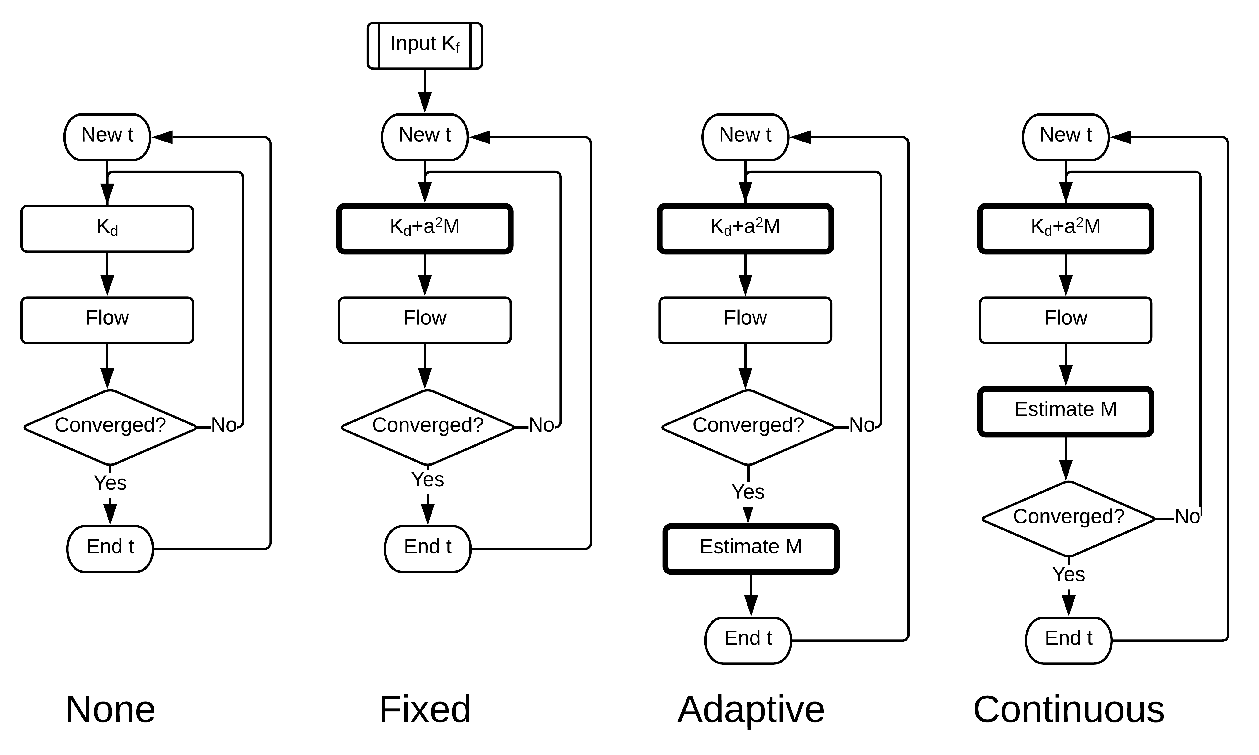
Four Variations of the Algorithm:
Numerical Experiments: Setup
1D quasi-static consolidation with a ramp-up load filled with a mixture of $H_2O$ and $CH_4$
- Verified against analytical solution for static poroelasticity
- Should get it exactly correct (if it's slow, stays linear, and we know $K_f$)
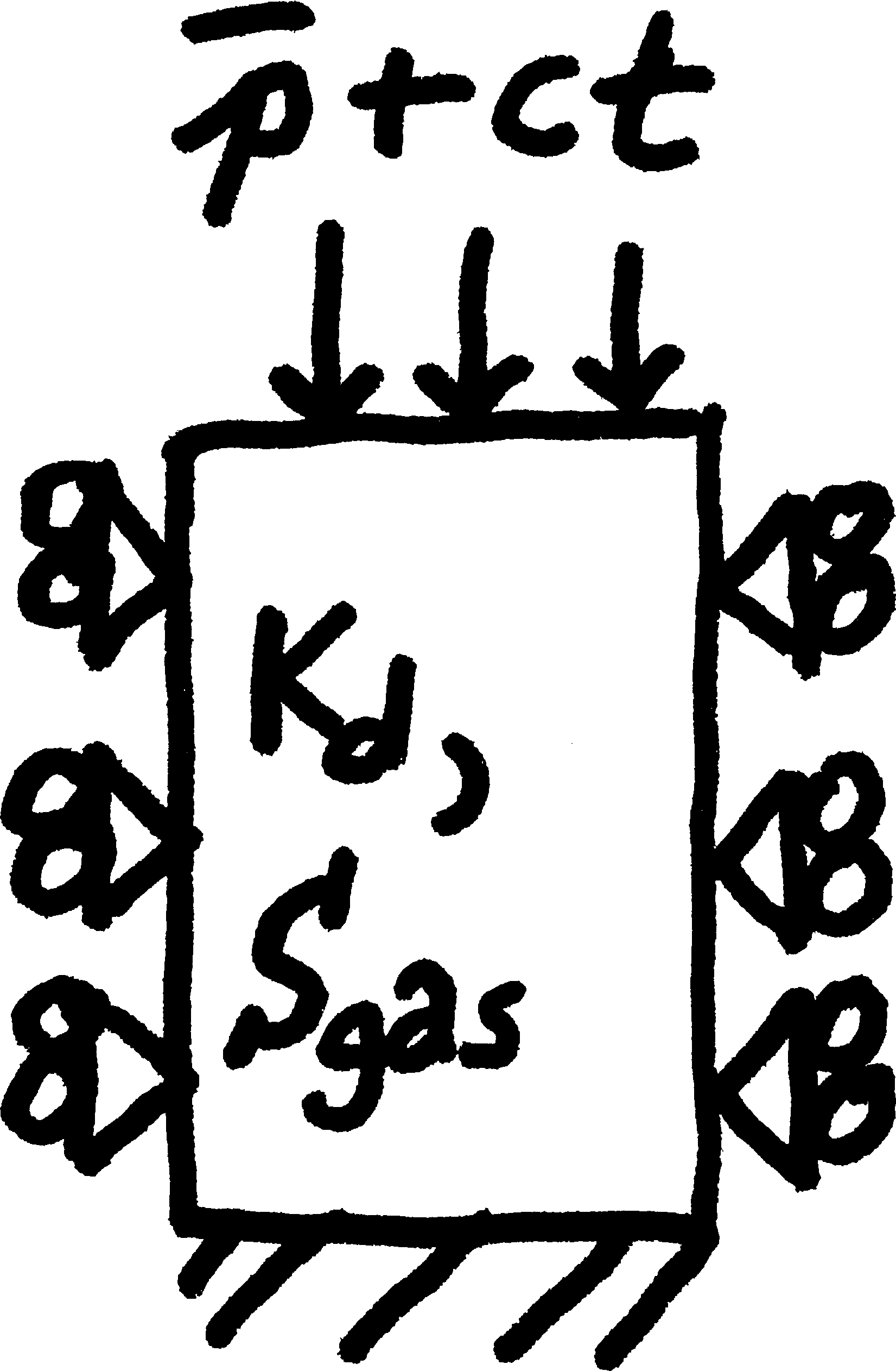
- Family of problems varied by:
- $K_ d$ skeletal stiffness
- $S_ {aqu}$ Water to gas ratio
- Algorithm is permuted by:
- Choice: None, Fixed, Adaptive, Continuous
- Tolerance on convergence
- Algorithm is evaluated by:
- Does it succeed
- Mean number of iterations for each set up
- Total runtime (too short)
Four Algorithms:
Numerical Experiments: Results
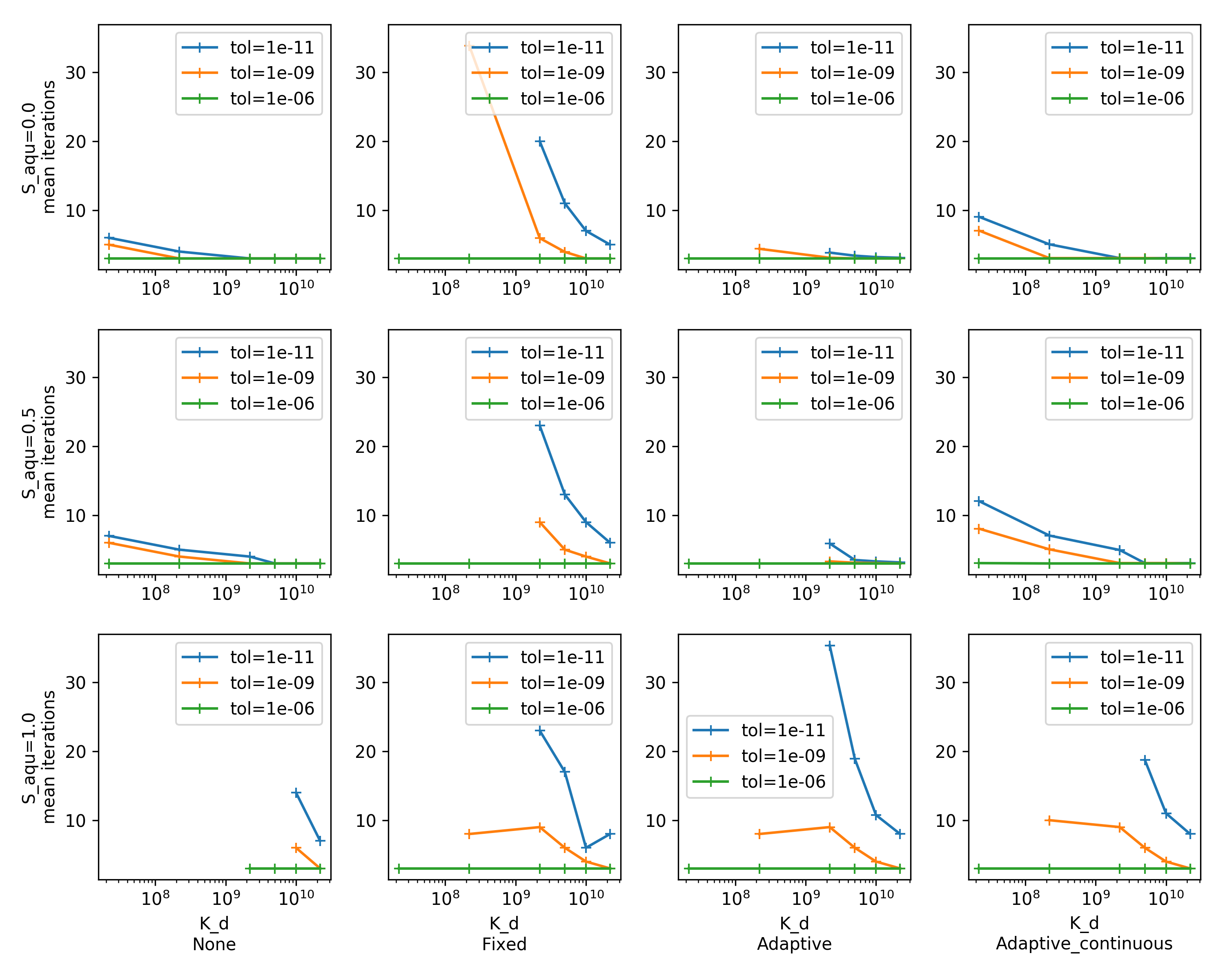
Each data point is one simulation; missing point reflects divergence.
Numerical Experiments: Results
- Original program with no preconditioning fails when $K_d < K_f$
- Fixed precondition solves that problem when $K_f$ was known
- Adaptation of $K_f^*$ upon convergence improves it
- Adapting during the time step iteration is robust for all compositions with reasonable tolerance
- Adapting can perform worse with gaseous pore fluids
- Algorithm estimates correct $K_f$ on this problem (not smooth in practice)
One more trick: under-relaxation
Algorithms work on 1D test problem, but still not 100\% robust in some reservoir problems.
Need to add under-relaxation: \begin{equation} \Delta u = [\mathtt{K}(K_d+\alpha^2 M^*)] \backslash \{\mathtt{R}(\sigma)\} \end{equation} And update by \begin{equation} u^{k+1} = u^k + \beta \Delta u \end{equation} With $0<\beta\leq 1$. Smaller $\beta$ slows down convergence.
Also, watch out for pore ``collapse'' when gases appear ($K_f \approx 50Pa$ vs $K_s \approx 10^{10} Pa$)
- Assumptions out of range for poroelastic porosity evolution?
Applications
All this work to get this type of problem to work:
Outro
- Hit divergence on coupled problems with drastic fluid compositional changes
- Appearance of gases makes staggered iteration raise
- Used poroelastic theory to design a way to adaptively precondition
- Permuted idea to make multiple staggering algorithms
- Tried all permutations on a simple constructed test problem
Comments:
- Look for places where our computer program is arbitrary and permute them.
- Design families of tiny test problems to program their limits
These sldies are hosted at: ocf.io/afq/slides/Siam2019
References:
Queiruga, Moridis, and Reagan, "Simulation of Gas Production from Multilayered Hydrate-Bearing Media with Fully Coupled Flow, Thermal, Chemical and Geomechanical Processes Using TOUGH+Millstone. Parts 1-3," Transport in Porous Media, 2019
Practices:
- Convergence difficult when $K_d \lessapprox K_f$ with naive approach
- Use unstructured quad meshes for mechanics
- True 2D axisymmetry for mechanics
- Continuous $M$ estimation for preconditioner
- Under relax $\Delta u$ by $\beta \approx 0.2-0.5$
- Timestep control: double below 25 and cutback at 100
- A lot of time per iteration, but stable on large timesteps.