Interactive ray made possible through a number of improvements to the renderer's efficiency including the use of the GPU.
Table of Contents
Part 0: Abstract
As the final project for CS184, I implemented ray tracing on the GPU. This involved several changes in order to make the renderer from project 3 suitable. Most prominently, I refactored recursive methods to be iterative and I used CUDA to write the GPU kernel. Finally, I wrote a BDPT version of the renderer in order to try to gain faster convergence of the renderer for scenes that can prove difficult for a classic path tracer such as in project 3.
This project was built on a Windows machine with a GeForce GTX 860M graphics card and Nsight Monitor Visual Studio Edition 5.1. Though I tried to make it cross platform, I have neither built nor tested it on any other machine. Additionally, the command line options for the program are not well tested. I just manipulated the defaults whenever I ran the program to set what I wanted to do. When you run the program it should prompt you with a file dialog if you haven't given it an input path. Just select the dae file you want.
This is discussed more below, but the program caches the processed dae files
it a format to make loading more efficient. If you change the dae file, you will
need to delete the cached files. They are located in the same folder as the dae
file and have the same name, but have the file type .dat or
.cam.dat added to the end.
Part 1: Technical Approach
Part 1.1: Iterative Rendering
The main goal of this project was to make a real time ray tracer. That meant that the ray tracer had to have a major speed up. The reference ray tracer was project 3's classic path tracer. It runs on the CPU, uses double precision, and ran all samples for a given area of the image before presenting the results.
In order to speed up the ray tracer, the last thing mentioned in that list was the first thing to change. Instead of running all the samples up front, the ray tracer runs over all pixels and sampling one ray for each. It then adds the sampled contributions to a grid of the totals. It then presents the grid divided by the number of times this has been executed to give the average contribution for each pixel. This is equivalent to the previous approach, but allows the user to see the progress as the renderer gathers more sampels. It also allows for the user to allow the renderer to run until it is converged.
This can be seen in pathtracer_kernel() in
c_pathtracer.cu. Specifically this code covers the core of this
logic.
bufferAccumulative[i] += spectrumFinal;
double3 col = bufferAccumulative[i] / (double)frameIndex;
float c = encodeColor(col);
bufferOutput[i] = make_float3(x, y, c);
Part 1.2: CUDA and the GPU
However this is still far to slow for interactivity. The CPU can't take advantage of the inherent parallelism of the problem like the GPU can. Thus, the next step was to move everything over to CUDA code in a GPU kernel.
Because I have an NVidia card, CUDA was the logical choice. This conversion required several changes. First all recursive code had to be changed to iterative solutions. This meant that I had to store the attenuation of the throughput, and then every time I interact with a surface, I would combine this into the attenuation.
Next, I had to convert the scene data into a form that could be used on the GPU. This meant that I had to convert materials, lights, primitives, and the BVH into a GPU friendly format. For the first two, I packed the information into a struct containing a union of the different types. This allowed for regularly packed information. These were placed into texture objects for faster lookup of the data[1].
The BVH had a similar treatment, but was stored in the texture object in a more efficient order. By linearizing the BVH tree in an order that allows nodes that are near each other to be near each other in memory, the GPU can take advantage of the spacial locality when traversing[2]. This is even better because when the intersection code is switched to an iterative version, it is apparent that the code would just go through the array from start to finish, perhaps skipping nodes, but never going backwards. This means that the GPU can take advantage of this when executing in parallel[3].
The primitives, including their vertices and normals, were done in a similar fashion. They were placed in the same order as the BVH so that intersections would be even faster.
Part 1.3: Floats
The next optimization was to change all doubles to floats. Though this does sacrafice some quality, this allows for much faster execution. The kernel ran on the order of four times faster when this was done. There are still some relics of the double code in the codebase, but they are all hidden by preprocessor flags.
This switch did prove to be difficult at first. Though it made the data much more compact in the texture objects. There were some accuracy errors that caused visual artifacts like striping on the walls. This was solved by subtracting an epsilon value from the ray lengths after an intersection was found. Previously, It was intersecting with an endpoint twice causing rays to be terminated when they shouldn't be. The floating point inaccuracies caused this occur.
Part 1.4: BDPT
The next step to making the renderer faster was implementing bidirectional
path tracing[4]. The core of this method is
located in pathtracer_trace_bidirectional_ray() in
c_pathtracer.cu. For each ray to sample, it grows a path from the
light and from the eye. It computes the throughput for that given path and
combines it. In order to do this on the GPU, and iterative growing of the path
up to a given maximum size allows for a static path array to be used. This
allows the GPU to optimize for a static stack size that can be precomputed via
static analysis. After the path throughputs are calculated, Veach proposes using
multiple importance sampling in order to fully optimize the minimization of
variance. Right now the implementation averages the samples for each path length
before combining them instead.
Part 1.5: Volumetrics
In order to test the improvements of this renderer over project 3, volumetric global fog was added to the renderer. This was done using an absorbtion and a scattering coefficient (\(\sigma_a\) and \(\sigma_s\) respectively) to figure out the probability of a ray traveling \(t\) units without interating. This is equal to \(e^{-t\cdot (\sigma_a + \sigma_s)}\). Using this equation, one can find that the distance a particle travels before interacting is equal to \(\frac{-\log(r)}{\sigma_a + \sigma_s}\) where \(r\) is a random number from 0 to 1. Using this, every time we test a ray for interacting with the scene, we generate a distance. If the distance is greater than whereever the ray hits a primitive in the scene, then the ray doesn't interact with the fog. Otherwise, the ray does interact with the fog at \(t\) units along its path.
If this happens, the random number is generated from 0 to 1. If it is greater than \(\frac{\sigma_s}{\sigma_a + \sigma_s}\), then the ray was absorbed and the path is terminated. Otherwise, the ray was scattered. To calculate the direction of the scattering, the Schlick Phase function was used because it is a faster approximation of the Henyey-Greenstein function. Where \(k\) is the bias for back (\(k=-1\)) and forward (\(k=1\)) scattering, the Schlick Phas function says that likelihood of a ray going in a given direction \(\theta\) is equal to the following
\[pdf(\theta)=\frac{1-k^2}{4\pi(1+k\cos\theta)^2}\]
Thus a ray on the uniform sphere is generated and the associated probability for the angle it makes with the original ray is used to generate a probability with which the throughput is attenuated.
Part 1.6: Gloss and Roughness
Glossy specularity was also implemented to test the renderer improvements. This effect was achieved by scattering the ray after it reflected or refracted by an amount based on its roughness. The code to do this follows.
rtrt_vec3 u = normalize(cross(rtrt_make_vec3(w.y, w.z, w.x), w));
rtrt_vec3 v = cross(u, w);
rtrt_vec3 sp = rtrt_uniform_hemisphere_sample(randState) * roughness;
sp.y += 1 - roughness;
w = sp.x * u + sp.z * v + sp.y * w;
The first step is to get two vectors that are orthogonal to each other and the original ray after it is reflected or refracted. This gives us a coordinate frame. We then generate a sample on a uniform hemisphere. By multiplying this sample by a roughness and then adding to the vertical direction based on the roughness, the sample is biased towards the unit y vector when roughness is closer to zero. This sample is then used with the orthogonal vectors to generate a biased sample that perturbs the original ray after reflection or refraction.
Part 1.7: Lessons Learned
The main thing that I learned through this project was that writing down the equations helped so much in understanding how they interact and work together. Understanding where solid angle and area integrals are being converted and how they are used together was very complicaated. Recording how I was using everything made it all much better.
Part 2: Results
Part 2.1: Specular
The following is a rendering of the reflective and refractive materials without roughness.
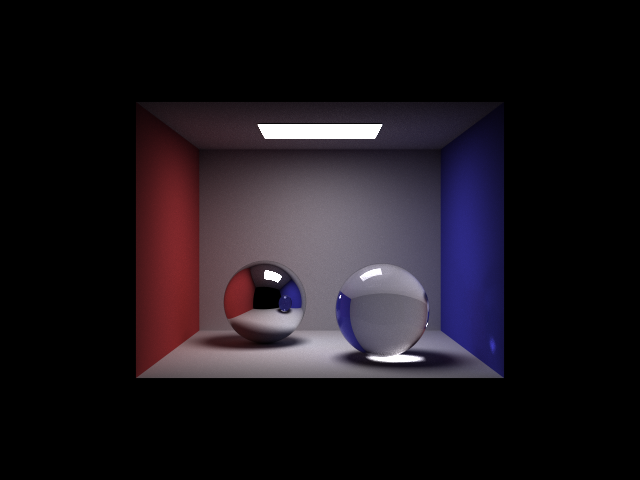
dae/sky/CBspheres.dae |
Part 2.2: Volumetric fog
The following is a rendering with volumetric fog on. The light was purple and the fog was white.
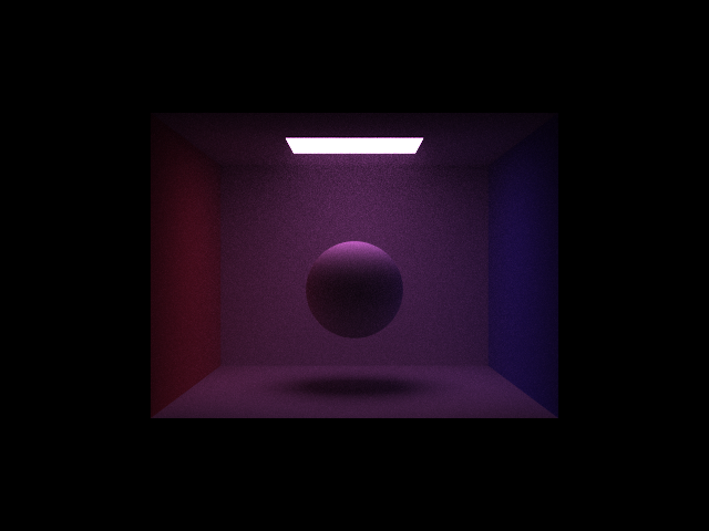
dae/sky/CBspheres_float.dae |
Part 2.3: Glossy
The following is a rendering of the reflective material with different roughnesses, though both are greater than 0.
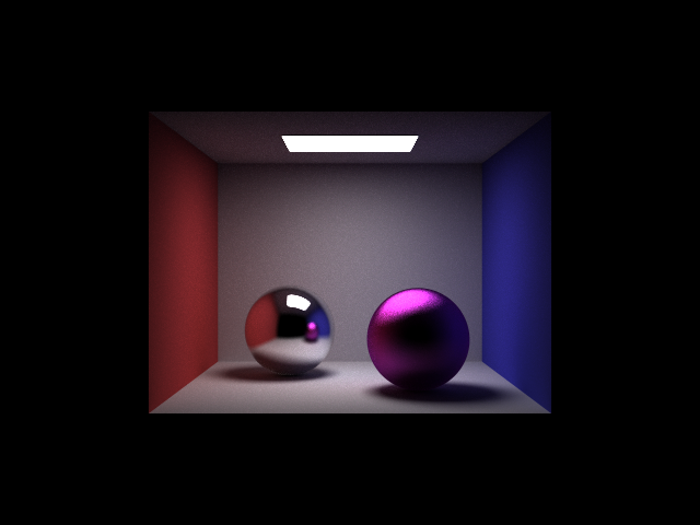
dae/sky/CBspheres_glossy.dae |