Introduction to neural networks with applications.
Introduction to convolutional neural networks with applications
Introduction to recurrent neural networks with applications.
4/05/2017
For today
Artificial Neural networks
Artificial Neural Network (ANN) or Neural Network (NN) are supervised machine learning classifiers
Based (loosely) on biological neural networks in the brain.
Origins of Neural Networks
Brain has many impressive features.
Parallelism.
Fast computation.
Ability to learn and generalize.
Simple operations are very complicated.
Origins of neural networks
Neural networks were designed to mimic the way the brain processes information.
Developmental periods: 1940s: Mcculloch and Pitts: Initial works 1960s: Rosenblatt: perceptrons, simple single layer NNs 1960s: Minsky and Papert: limitations of perceptrons 1980s: Hopfield/Werbos and Rumelhart: Hopfield's energy approach/back-propagation learning algorithm
Biological neural networks

Biological neural networks
Signal reaches a synapse: releases chemicals called neurotransmitters
Cerebral cortex: a large flat sheet of neurons about 2 to 3 mm thick and 2200cm , \(10^{11}\) neurons
Duration of impulses between neurons: milliseconds and the amount of information sent is also small(few bits)
Critical information are not transmitted directly , but stored in interconnections
Connectionist model initiated from this idea.
Mucollough-Pitts model

Neural networks overview

Neural networks overview

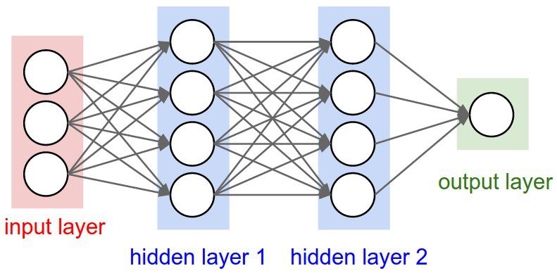
Feedforward networks
Activation functions

Feedforward example

Learning in neural networks: backpropagation
How are weights estimated?
Algorithm known as backpropagation – combination of stochastic gradient descent and use of the chain rule.
Learning in neural networks: backpropagation algorithm
Random initialization of weights for inputs.
Estimation of predicted values and calculation of the cost function: \(E = \frac{1}{2} \sum_{i=1}^{N} ||y_{i}-\hat{y}_{i}||^{2}\)
Estimate gradient of each weight in the network wrt to the cost function: \(\nabla E = \left(\frac{\partial E}{\partial w_{1}}, \frac{\partial E}{\partial w_{2}} , \cdots \right)\)
Update the weights in the direction of the negative gradient \(-\gamma\frac{\partial E}{\partial w_{i}}\) with learning rate \(\gamma\) and repeat.
Backpropagation learning

General applications
Digital charachter recognition.
Image compression.
Stock market prediction.
Medical diagnoses etc.
Social science applications
Any supervised learning problem.
Predicting elections.
Text classification.
Time series prediction.
Neural Networks in R: Predicting Breast Cancer
# Wisconsin Breast Cancer Database
library(mlbench)
data(BreastCancer)
dim(BreastCancer)
## [1] 699 11
levels(BreastCancer$Class)
## [1] "benign" "malignant"
head(BreastCancer)
##        Id Cl.thickness Cell.size Cell.shape Marg.adhesion Epith.c.size
## 1 1000025            5         1          1             1            2
## 2 1002945            5         4          4             5            7
## 3 1015425            3         1          1             1            2
## 4 1016277            6         8          8             1            3
## 5 1017023            4         1          1             3            2
## 6 1017122            8        10         10             8            7
##   Bare.nuclei Bl.cromatin Normal.nucleoli Mitoses     Class
## 1           1           3               1       1    benign
## 2          10           3               2       1    benign
## 3           2           3               1       1    benign
## 4           4           3               7       1    benign
## 5           1           3               1       1    benign
## 6          10           9               7       1 malignant
Neural Networks in R: Predicting Breast Cancer
# Wisconsin Breast Cancer Database
head(BreastCancer)
##        Id Cl.thickness Cell.size Cell.shape Marg.adhesion Epith.c.size
## 1 1000025            5         1          1             1            2
## 2 1002945            5         4          4             5            7
## 3 1015425            3         1          1             1            2
## 4 1016277            6         8          8             1            3
## 5 1017023            4         1          1             3            2
## 6 1017122            8        10         10             8            7
##   Bare.nuclei Bl.cromatin Normal.nucleoli Mitoses     Class
## 1           1           3               1       1    benign
## 2          10           3               2       1    benign
## 3           2           3               1       1    benign
## 4           4           3               7       1    benign
## 5           1           3               1       1    benign
## 6          10           9               7       1 malignant
Neural Networks in R: Predicting Breast Cancer
Remove missing data
apply(BreastCancer,2,function(x) sum(is.na(x)))
##              Id    Cl.thickness       Cell.size      Cell.shape
##               0               0               0               0
##   Marg.adhesion    Epith.c.size     Bare.nuclei     Bl.cromatin
##               0               0              16               0
## Normal.nucleoli         Mitoses           Class
##               0               0               0
BreastCancer<-na.omit(BreastCancer)
Divide the data into test and training (75/25)
index <- sample(1:nrow(BreastCancer),round(0.75*nrow(BreastCancer)))

Cancer<-ifelse(BreastCancer$Class == "malignant", 1,0)
Prepare the data for neural network analysis
Scaling is the most important thing to do
data<-data.matrix(BreastCancer[,2:10]) # transforms to numeric
maxs <- apply(data, 2, max)
mins <- apply(data, 2, min)

scaled <- scale(data, center = mins, scale = maxs - mins)

trainX <- data.frame(scaled[index,])
testX <- data.frame(scaled[-index,])
trainY<-Cancer[index]
testY<-Cancer[-index]
Train the neural network in R
library(neuralnet)
n <- names(trainX)
f<-paste(n,collapse = " + ")
f <- as.formula(paste("trainY~",f))
nn <- neuralnet(f,data=trainX,
                hidden = c(3),
                act.fct = "logistic")
plot(nn)
Train the neural network in R

Predict data on test set
pr.nn <- compute(nn,testX)
head(pr.nn$net.result)
##              [,1]
## 1  0.003779671987
## 3  0.003779722914
## 19 1.003092096916
## 29 0.003779723021
## 31 0.003779722951
## 32 0.003779722985
these are the predicted values of the test set
These need to be transformed into predictions
Create confusion matrix and calculate accuracy, specificity and sensitivity
predictions<-ifelse(pr.nn$net.result > .5, 1,0)
confusion = table(testY,predictions)
confusion
##      predictions
## testY   0   1
##     0 106   5
##     1   4  56
Create confusion matrix and calculate accuracy, specificity and sensitivity
accuracy<-c(confusion[1,1]+confusion[2,2])/sum(confusion)
accuracy
## [1] 0.9473684211
specificity<-confusion[1,1]/sum(confusion[1,])
specificity
## [1] 0.954954955
sensitivity<-confusion[2,2]/sum(confusion[2,])
sensitivity
## [1] 0.9333333333
Image classification and convolutional neural networks
A special type of neural network called convolutional neural networks (CNNs) are very useful for image classification.
To understand how they work, we must understand what an image is.
How does a computer see an image?
Images represented as a matrix of pixels.
Each image is represented in a machine as a matrix of pixels.
Entries of each matrix contain pixel intensity values which are integers that range in numbers from [0,255].
Color images are represented as three matrices of pixel intensity values

- One for each channel: Red, Green and Blue.
Black and white images are represented as three matrices of pixel intensity values
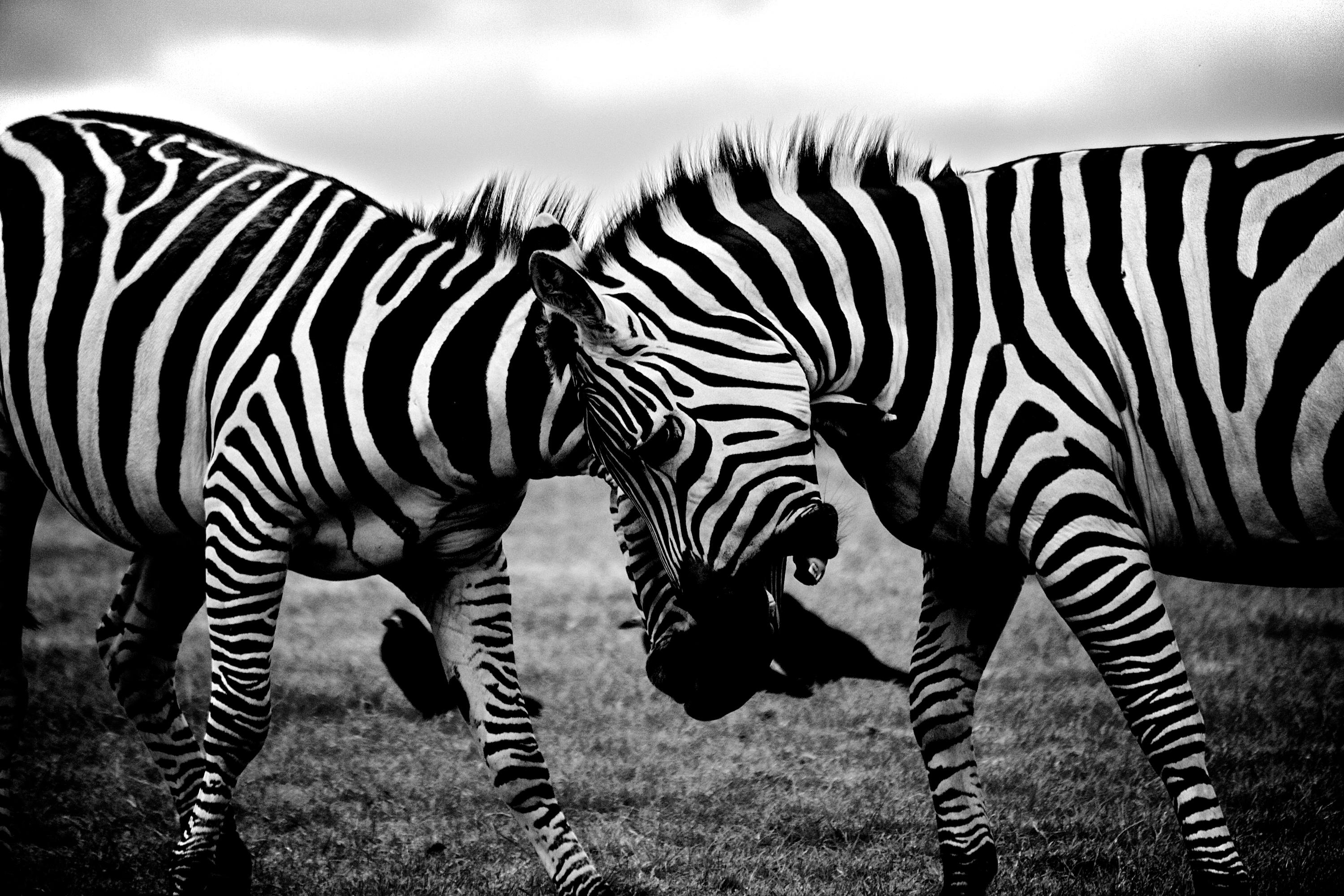
Image classification
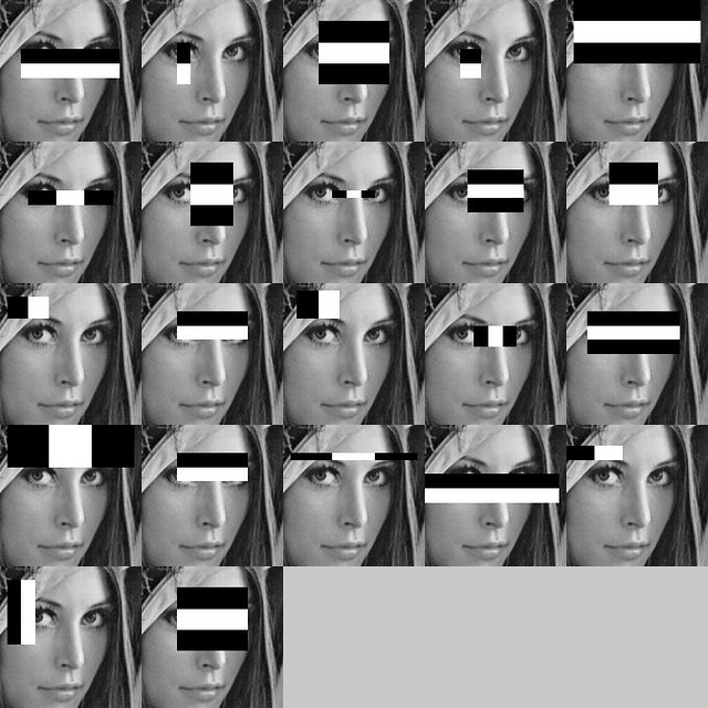
Past approached to image classification involved detecting geometry in images.
Cubes, facial features etc.
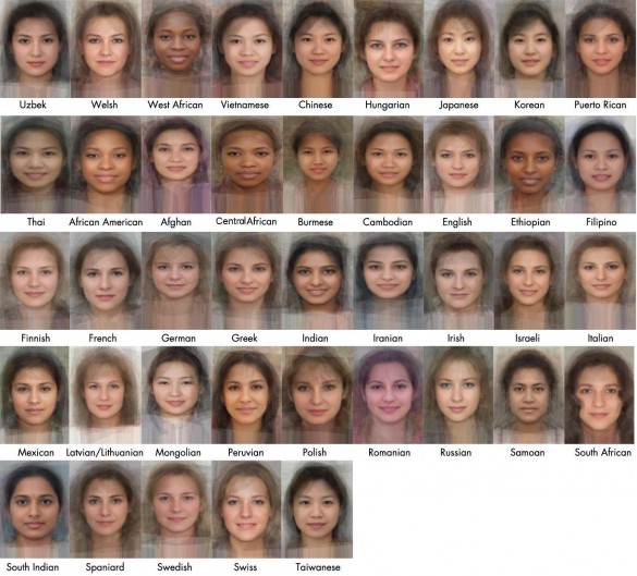
Viola-jones algorithm & haarcascades for detecting faces.
Generally very difficult to detect other object in images.
Because of occlusions, differences in lighting, deformations etc, it is very difficult to detect features in images.
Requires answering the Platonic question: what is a chair? What is a car etc.
Data driven methods
With better computing power and more, data we can successfully classify images using only the pixel data.
Convolutional neural networks, which convolve (slide) the classifier across the pixel data, have been found to be most successful
Convolutional neural networks

Convolutional Neural Networks Tutorial in R: Predicting Race