Getting the most out of topic modeling.
Multidimensional scaling of texts.
Introduction to Computer Vision and Image Analysis
4/05/2017
For today
Getting the most out of topic models
Topic models give us two types of outputs that allow us to do many things.
Output 1: topics in a corpus.
Output 2: topic proportions for each document.
Topics in a corpus - corpus structure
Estimating a topic model over a corpus allows us to get a sense of how a set of docs are structured.
Let's do an example with the Associated Press articles
Associated press articles
data("AssociatedPress")
AssociatedPress
## <<DocumentTermMatrix (documents: 2246, terms: 10473)>>
## Non-/sparse entries: 302031/23220327
## Sparsity           : 99%
## Maximal term length: 18
## Weighting          : term frequency (tf)
ap_lda <- LDA(AssociatedPress, k = 5, control = list(seed = 1234))

# Getting the most out of topic models.

terms(ap_lda, k=10) # top 10 words for each topic
##       Topic 1      Topic 2      Topic 3   Topic 4  Topic 5
##  [1,] "percent"    "bush"       "million" "i"      "government"
##  [2,] "year"       "soviet"     "new"     "people" "police"
##  [3,] "million"    "president"  "company" "two"    "court"
##  [4,] "billion"    "i"          "market"  "police" "people"
##  [5,] "new"        "united"     "stock"   "years"  "two"
##  [6,] "report"     "states"     "billion" "new"    "state"
##  [7,] "last"       "new"        "percent" "three"  "case"
##  [8,] "years"      "house"      "year"    "city"   "years"
##  [9,] "workers"    "dukakis"    "york"    "like"   "south"
## [10,] "department" "government" "dollar"  "school" "attorney"
Let's name topics 1-5
terms(ap_lda, k=15) # top 10 words for each topic
##       Topic 1      Topic 2      Topic 3   Topic 4    Topic 5
##  [1,] "percent"    "bush"       "million" "i"        "government"
##  [2,] "year"       "soviet"     "new"     "people"   "police"
##  [3,] "million"    "president"  "company" "two"      "court"
##  [4,] "billion"    "i"          "market"  "police"   "people"
##  [5,] "new"        "united"     "stock"   "years"    "two"
##  [6,] "report"     "states"     "billion" "new"      "state"
##  [7,] "last"       "new"        "percent" "three"    "case"
##  [8,] "years"      "house"      "year"    "city"     "years"
##  [9,] "workers"    "dukakis"    "york"    "like"     "south"
## [10,] "department" "government" "dollar"  "school"   "attorney"
## [11,] "federal"    "campaign"   "bank"    "time"     "last"
## [12,] "prices"     "party"      "inc"     "just"     "trial"
## [13,] "program"    "committee"  "trading" "children" "judge"
## [14,] "government" "congress"   "corp"    "first"    "officials"
## [15,] "oil"        "reagan"     "share"   "day"      "prison"
Which documents were in which topics?
- This gives us a NxK matrix of the topic proportions for each documents
posterior_inference <- posterior(ap_lda)
posterior_topic_dist<-posterior_inference$topics # This is the distribution of topics for each document
dim(posterior_topic_dist)
## [1] 2246 5
Which documents were in which topics?
- It's easy to find which documents had the highest probability for topic 2
topic_2_docs<-which(posterior_topic_dist[,2] > 0.50)
topic_2_docs[1:10]
## [1] 2 6 8 13 14 18 27 32 39 50
Let's look at some of the words in two documents from the same topic
library(tidytext)
ap_td <- tidy(AssociatedPress)
wordcloud(sample(ap_td[ap_td$document==6,]$term,10), xlab = "Document 6")
## Warning in wordcloud(sample(ap_td[ap_td$document == 6, ]$term, 10), xlab =
## "Document 6"): strongman could not be fit on page. It will not be plotted.
## Warning in wordcloud(sample(ap_td[ap_td$document == 6, ]$term, 10), xlab =
## "Document 6"): achieve could not be fit on page. It will not be plotted.

Let's look at some of the words in two documents from the same topic
wordcloud(sample(ap_td[ap_td$document==8,]$term,10), xlab = "Document 8")
## Warning in wordcloud(sample(ap_td[ap_td$document == 8, ]$term, 10), xlab =
## "Document 8"): democratic could not be fit on page. It will not be plotted.
## Warning in wordcloud(sample(ap_td[ap_td$document == 8, ]$term, 10), xlab =
## "Document 8"): growing could not be fit on page. It will not be plotted.

What % of documents fall under each topic?
To understand more about a corpus we might be interested in what % of documents fall under each topic.
This is especially useful for understanding things like news coverage.
Here, we can find out (roughly), what % of Associated Press articles are in each topic.
How much coverage did the Associated Press devote to each topic?
pct_topic1<-length(topic_1_docs)/dim(posterior_topic_dist)[1]
pct_topic2<-length(topic_2_docs)/dim(posterior_topic_dist)[1]
pct_topic3<-length(topic_3_docs)/dim(posterior_topic_dist)[1]
pct_topic4<-length(topic_4_docs)/dim(posterior_topic_dist)[1]
pct_topic5<-length(topic_5_docs)/dim(posterior_topic_dist)[1]

Coverage<-c(pct_topic1,pct_topic2,pct_topic3,pct_topic4,pct_topic5)
Topics<-c("Topic 1", "Topic 2","Topic 3","Topic 4","Topic 5")
plot(Coverage)
text(1:5,y=Coverage,labels=Topics)

Document similarity
\[ document-similarity = \sum_{k=1}^{K}\left(\sqrt{\theta_{d,k}} + \sqrt{\theta_{f,k}}\right)^2 \] - Topic proportions from topic models can also be used to compare documents by how similar they are.
Document similarity function
doc_similarity<-function(doc1,doc2){
  sim<-sum(
    (sqrt(doc1) + sqrt(doc2))^2
  )
  return(sim)
}
Using topic proportions, calculate AP article similarity
- Let's figure out which article is most similar to article 1.
similarity_scores<-c(0)

for(i in 2:dim(posterior_topic_dist)[1]){
  similarity_scores<-c(similarity_scores,
      doc_similarity(posterior_topic_dist[1,], posterior_topic_dist[i,]))
}

which.max(similarity_scores)
## [1] 1523
Using topic proportions, calculate AP article similarity
It seems as if article 1523 is the most similar.
What words does it have?
Using topic proportions, calculate AP article similarity
par(mfrow = c(1,2))
wordcloud(sample(ap_td[ap_td$document==1,]$term,10))
## Warning in wordcloud(sample(ap_td[ap_td$document == 1, ]$term, 10)):
## classroom could not be fit on page. It will not be plotted.
## Warning in wordcloud(sample(ap_td[ap_td$document == 1, ]$term, 10)): family
## could not be fit on page. It will not be plotted.
## Warning in wordcloud(sample(ap_td[ap_td$document == 1, ]$term, 10)): shot
## could not be fit on page. It will not be plotted.
## Warning in wordcloud(sample(ap_td[ap_td$document == 1, ]$term, 10)): susan
## could not be fit on page. It will not be plotted.
wordcloud(sample(ap_td[ap_td$document==1523,]$term,10))
## Warning in wordcloud(sample(ap_td[ap_td$document == 1523, ]$term, 10)):
## efforts could not be fit on page. It will not be plotted.
## Warning in wordcloud(sample(ap_td[ap_td$document == 1523, ]$term, 10)):
## knows could not be fit on page. It will not be plotted.
## Warning in wordcloud(sample(ap_td[ap_td$document == 1523, ]$term, 10)):
## working could not be fit on page. It will not be plotted.
## Warning in wordcloud(sample(ap_td[ap_td$document == 1523, ]$term, 10)):
## criticism could not be fit on page. It will not be plotted.
## Warning in wordcloud(sample(ap_td[ap_td$document == 1523, ]$term, 10)):
## teaching could not be fit on page. It will not be plotted.

Document clustering and multidimensional scaling
We are often interested in finding out how similar a set of documents are for a variety of reasons.
May be interested in identifying latent features of document.
May be interested in scoring documents to see how these scores relate to other features of the documents.
Hierarchical Clustering (HC)
As the name suggest HC builds a hierarchy of clusters.
Two types of hierarchical clustering:
Agglomerative - "Bottom up". Each observation has its own unique cluster, clusters are merged based on distance metrics.
Divisive - "Top down" - each observation is assumed to be in its own cluster and clusters are broken apart.
Hierarchical clustering algorithm
HC, like multidimensional scaling, is a clustering method that is based on some measure of "distance" between two observations.
Algorithm proceeds by grouping observations by distance.
Types of distance
Euclidean
\[\|x_{1}-x_{2} \|_2 = \sqrt{\sum_i (x_{1i}-x_{2i})^2}\]
Types of distance
Squared Eudlidean
\[\|x_{1}-x_{2} \|_2^2 = \sum_i (x_{1i}-x_{2i})^2\]
Types of distance
Manhattan
\[\|x_{1}-x_{2} \|_1 = \sum_i |x_{1i}-x_{2i}|\]
- etc
Linkage criterion and dendrograms
Hierarchical clustering proceeds by clustering observations based on linkage criterion.
This is essentially the maximum distance between sets of observations.
Ward's criterion proceeds by creating clusters based on within-cluster variance minimization.
This is what we use below to cluster Trump's tweets
Clustering with the Iris Dataset
data(iris)
d<-dist(iris)
## Warning in dist(iris): NAs introduced by coercion
#run hierarchical clustering using Ward’s method
clusters <- hclust(d,method="ward.D")
# Plot the dendrogram to figure out how many clusters
plot(clusters, hang=-1)

Clustering with the Iris Dataset
- Clear separation between each species
First 100 of Trumps tweets
# Create a distance object using the dtm
d<-dist(dtm_mat)
#run hierarchical clustering using Ward’s method
clusters <- hclust(d,method="ward.D")
# Plot the dendrogram to figure out how many clusters
plot(clusters, hang=-1)

Interpreting the dendrogram
- Looking at the dendrogram, we have to figure out how many clusters there are based on how well the tree separates.
Dendrogram of Trump's Tweets
plot(clusters, hang=-1,main="Dendrogram of Trump's Tweets")

Label documents
Looks like we have two well separated clusters here.
We can now label the documents by cutting the tree.
cluster_labels<-cutree(clusters,k=2)
cluster_labels[1:10]
##  1  2  3  4  5  6  7  8  9 10
##  1  1  1  1  1  1  1  1  1  1
Label documents
hist(cluster_labels)

What do these clusters look like?
par(mfrow=c(1,2))
wordcloud(cat_1_tweets)
wordcloud(cat_2_tweets)

Multidimensional Scaling
There are occasions in which we might be interested in scoring documents on how similar they are.
This can be done by performing multidimensional scaling on the Document-Term Matrix.
Multidimensional Scaling of Members of Congress
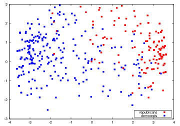
Multidimensional Scaling of Members of Congress
This is accomplished by collapsing the matrix of roll call votes
Members of Congress are rows (observations)
Bills voted on are columns.
Multidimensional Scaling
Like hierarchical clustering, scoring based on distance between observations
Researcher must chose the number of dimensions they belive the data fall along.
Multidimensional Scaling
d <- dist(dtm_mat) # euclidean distances between the rows
fit <- cmdscale(d,eig=TRUE, k=2) # k is the number of dim
fit # view results
## $points
##             [,1]          [,2]
## 1   -0.109514564 -0.1645042703
## 2   -0.442949095 -0.4960486696
## 3   -0.837521872 -0.8659574302
## 4   -0.608086405 -0.0970066432
## 5   -1.102867856 -1.1016083832
## 6   -0.724936662 -0.8169614035
## 7   -0.511169283 -0.4561615039
## 8   -0.192213224 -0.2468884902
## 9   -0.540490306 -0.3541473328
## 10  -0.197609572 -0.2739829020
## 11  -0.305545899 -0.3306166888
## 12  -0.036719257 -0.0080872906
## 13   0.198144897  0.2144453488
## 14  -0.453019233 -0.6312600792
## 15   0.942690568  0.1217700976
## 16  -0.107850542  0.9039900031
## 17   0.812430590  0.9586734290
## 18   0.136668509  1.2136884719
## 19   2.524500400 -0.9470032759
## 20  -0.032135534  0.9251504344
## 21   0.039872738 -0.1665159093
## 22  -0.278654347  0.3406534790
## 23   1.472442907 -0.6441975873
## 24  -0.054083716 -0.2245602515
## 25  -0.166526559 -0.1568424456
## 26  -0.143283609  0.5718079263
## 27   0.079930283  0.8435121480
## 28   0.388767120 -0.1604193262
## 29  -0.239730197  1.2769651927
## 30   1.457873398 -0.7090279713
## 31  -0.030729702 -0.1498532818
## 32  -0.888416260 -1.0361411273
## 33  -0.660291595 -0.5248479180
## 34  -0.169750981  0.9006137152
## 35   0.012414911  1.7097589527
## 36  -0.144941258  0.8178215705
## 37  -0.178302379  0.2274335631
## 38  -0.937548019 -1.1090456650
## 39   1.845928626 -0.8503936835
## 40  -0.020844638  0.6858900874
## 41  -0.162889312 -0.3280361374
## 42  -0.255717851 -0.3713366152
## 43  -0.948105238 -1.1033829867
## 44   0.039148090  0.6375745427
## 45  -0.457655471 -0.6466236538
## 46  -1.053201959 -0.6295670366
## 47   0.049648069 -0.1546592396
## 48   0.047486733  0.8144082865
## 49   0.061730094  0.1316096120
## 50  -0.030365597 -0.1624289641
## 51  -0.092876844  0.9788446336
## 52   0.039059673  0.7339423083
## 53   0.001154749  0.8943415458
## 54  -0.833113949 -0.7532062116
## 55  -0.267791423  1.2656499795
## 56  -0.697207526  0.1508921500
## 57   0.107105048 -0.4298716804
## 58   0.335362800  0.0021570705
## 59   1.497380323 -0.7266736197
## 60   1.507368853  0.0261593949
## 61  -0.325378062  0.8231606009
## 62  -0.140107109  0.4643170541
## 63  -0.159269531  0.2926661125
## 64   1.657569240 -0.7573984104
## 65   0.055817572 -0.0009525842
## 66   0.035148691  0.6214167227
## 67   0.096433781  0.1218501419
## 68   0.715643217 -0.1776254469
## 69   0.118522049 -0.3642100233
## 70  -0.024650314  0.1865721952
## 71   1.821510830 -0.8526321165
## 72  -0.049562494  0.3223530970
## 73   1.189023893 -0.5355078323
## 74  -0.059303771  0.6614964396
## 75  -0.005729447 -0.1762334642
## 76  -0.011712623  0.0220981623
## 77  -0.099771179 -0.0040304081
## 78   0.174848049  0.6704131625
## 79  -1.014007242 -1.3808579586
## 80  -0.332241034 -0.3514666609
## 81  -0.347813928 -0.3023879284
## 82  -0.195247120  0.9611058186
## 83  -0.025371219  0.5903325980
## 84  -0.020754135  0.9125767107
## 85  -0.125498445  0.1166766763
## 86  -0.824117675 -1.0556502667
## 87  -0.629956669  0.4074952973
## 88  -0.917737223 -0.8471116441
## 89  -0.394559336 -0.0593205884
## 90  -0.036602800  0.0106188929
## 91  -0.057910973 -0.0038961750
## 92  -0.145871210  0.2327355335
## 93  -0.037352786  1.0030126125
## 94   0.937586850 -0.4185732040
## 95  -0.723968204 -0.3711360408
## 96  -0.351191771 -0.4692103411
## 97  -0.067190852  0.8403889182
## 98   0.260718788 -0.1538084099
## 99   0.424178117 -0.2274740762
## 100  0.953424429 -0.2716914353
##
## $eig
##   [1] 4.471857e+01 4.249156e+01 3.610639e+01 3.529791e+01 2.972349e+01
##   [6] 2.882576e+01 2.517096e+01 2.438209e+01 2.337195e+01 2.262643e+01
##  [11] 2.220507e+01 2.105077e+01 2.042574e+01 1.971799e+01 1.943795e+01
##  [16] 1.892194e+01 1.785974e+01 1.743737e+01 1.697382e+01 1.681501e+01
##  [21] 1.621299e+01 1.590442e+01 1.568502e+01 1.538055e+01 1.513455e+01
##  [26] 1.466049e+01 1.453625e+01 1.405817e+01 1.390721e+01 1.366779e+01
##  [31] 1.327558e+01 1.302643e+01 1.277306e+01 1.234326e+01 1.204553e+01
##  [36] 1.188556e+01 1.160865e+01 1.153547e+01 1.117040e+01 1.101355e+01
##  [41] 1.083553e+01 1.050162e+01 1.038432e+01 1.035352e+01 1.022762e+01
##  [46] 1.005158e+01 9.894444e+00 9.775085e+00 9.606719e+00 9.554553e+00
##  [51] 9.446657e+00 9.315596e+00 9.240618e+00 9.137575e+00 8.871197e+00
##  [56] 8.663607e+00 8.548609e+00 8.339425e+00 8.215678e+00 8.025499e+00
##  [61] 7.836584e+00 7.669669e+00 7.574135e+00 7.461736e+00 7.311643e+00
##  [66] 7.118010e+00 7.091135e+00 6.794390e+00 6.769507e+00 6.607851e+00
##  [71] 6.440378e+00 6.418518e+00 6.295144e+00 6.072078e+00 6.000771e+00
##  [76] 5.868632e+00 5.719767e+00 5.594842e+00 5.452148e+00 5.410268e+00
##  [81] 5.057579e+00 5.024931e+00 4.945905e+00 4.871613e+00 4.648680e+00
##  [86] 4.573926e+00 4.447906e+00 4.351145e+00 4.063875e+00 3.899965e+00
##  [91] 3.838825e+00 3.626396e+00 3.386404e+00 3.273121e+00 2.891540e+00
##  [96] 2.764230e+00 2.711292e+00 2.424566e+00 9.459804e-01 1.705928e-14
##
## $x
## NULL
##
## $ac
## [1] 0
##
## $GOF
## [1] 0.07481803 0.07481803
Plot first and second dimensions
Dim1 <- fit$points[,1]
Dim2 <- fit$points[,2]

plot(Dim1, Dim2, xlab="First Dimension", ylab="Second Dimensions",
  main="Metric  MDS",   type="n")
text(Dim1, Dim2, labels = row.names(dtm_mat), cex=.7)
