In general, the purpose of unsupervised learning is dimensionality reduction
Discovery of latent dimensions given some data.
Examples) K-means clustering, principal components analysis, multidimensional scaling, EM algorithm.
3/16/2017
Unsupervised Learning with Text
K-means clustering

K-means clustering iteratively finds "groupings" of data using random intialization of clusters.
Applications: discovering latent groupings from data (ideological viewpoints, etc), learning features from images etc.
Closely related to EM algorithm which will be discussed later.
Principal components analysis
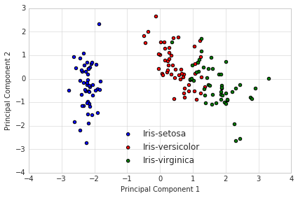
Uses matrix factorization to extract top "factors" that explain the most variance in the data.
Applications - construction of latent dimensions from a large group of items (eg psychometrics)
Multidimensional Scaling

- Multidimensional scaling via the NOMINATE procedure, short for "Nominal Three-Step Estimation" is similar to PCA and functions as a means of collapsing large matrices of vote data into two left right dimensions.
Unsupervised learning for text data
In general, we are interested in learning about latent similarities between documents.
Applications: are the issues that presidents write executive orders for different? do experimental treatments change the issues discussed in open ended surveys? how are speeches by Republicans and Democrats different?
Unsupervised learning methods for text data
Latent semantic analysis - uses singular value decomposition (linera algebra) to measure similarity between documents.
K-means clustering - uses K-Means algorithm to measure similarity between documents.
Topic modeling - uses nonparametric Bayesian model to measure similarity between documents and measure topics.
Topic models: Motivation
What are the topics that a document is about?
Given one document, can we find other documents about the same topics?
How do topics change over time?
Flavors of topic models: correlated topic models, structural topic models, dynamic topic models, semi-supervised topic models.
Nonparametric Bayesian modeling
- Topic models are generative which means that they model texts as if they were generated from a certain probability distribution.
-Each document defines a distribution over (hidden) topics.
-Assume each topic defines a distribution over words.
-The posterior probability of latent variables given a corpus determines the collection into topics
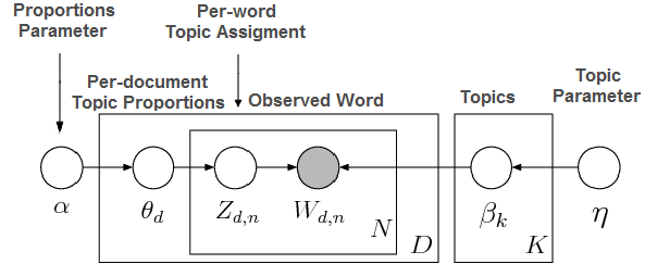
The generative model
\(D = \{d_{1},\cdots,d_{n}\}\) documents contain a vocabulary of \(V = \{v_{1},\cdots,v_{w}\}\) terms.
Assume \(K\) topics (pre-specified).
Each document has \(K\)-dimensional multinomial \(\theta_{d}\) over topics with a common Dirichlet prior \(Dir(\alpha)\)
Each topic has a \(V\)-dimensional multinomial \(\beta_{k}\) over words with a common symmetric Dirichlet prior \(D(\eta)\).
What does a Dirichlet look like?

Dirichlet expresses probabilities on an N-dimensional simplex.
Parameters are vectors of length K or V, respectively such that: \(\alpha,\eta \in \mathbb{R}^+\)
Generative process
For each topic \(1 \cdots k\): 1. Multinomial over words \(\beta_{k} \sim Dir(\eta)\)
For each document \(1\cdots d\):
- Multinomial over topics \(\theta_{d} \sim Dir(\alpha)\)
2 For each word \(w_{d,n}\): a. Draw topic \(Z_{d,n}\sim Mult(\theta_{d})\) with \(Z_{d,n}\in [1..K]\) b. Draw a word \(w_{d,n}\sim Mult(Z_{d,n})\)
Generative process
Generative process
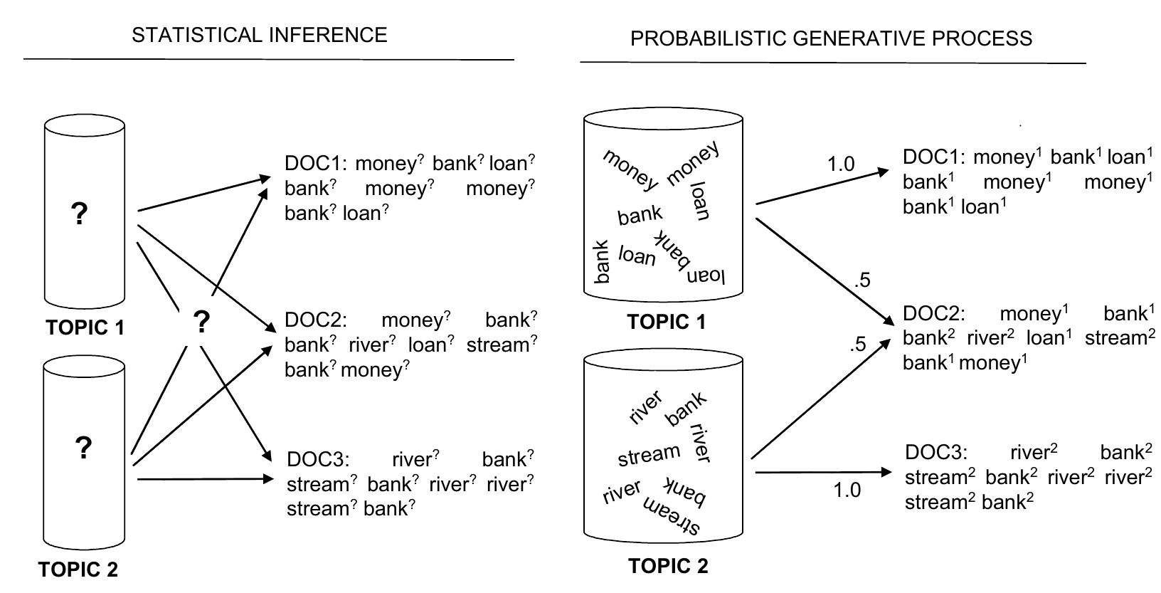
Inference problem
\[ \displaystyle P(\theta, z,\beta| w,\alpha,\eta) = \frac{P(\theta, z, \beta ; w,\alpha,\eta)}{\int\int \sum P(\theta,z,\beta, w,\alpha,\eta)} \] - Cannot do integral in the denominator
- Need to use approx. inference (1) Gibbs sampling ; (2) variational inference
Quantiaties we need to calculate
- Gibbs sampling aside, as Bayesians we need to calculate expected values of the parameters given the data.
Topic probability of word v according to topic k: \[\bar{\beta}_{k,v} = E[\beta_{k,v}|w_{1:D,1:N}] \] Topic proportions of each document d: \[\bar{z}_{d,n,k} = E[Z_{d,n} = k|w_{1:D,1:N}] \]
Topic assignment of each word \(w_{d,n}\): \[\bar{\theta}_{k,v} = E[\theta_{d,k}|w_{1:D,1:N}] \]
Visualizing a topic
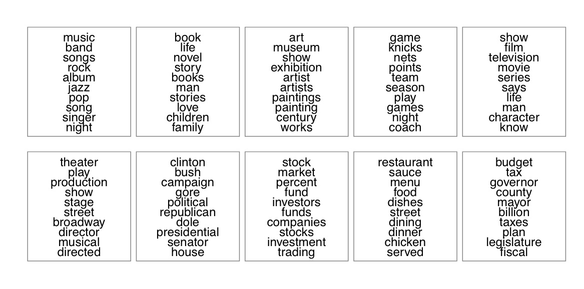
- Rank words in topics using highest term score.
Visualizing a document

Comparing similarity between documents
\[ document-similarity = \sum_{k=1}^{K}\left(\sqrt{\theta_{d,k}} + \sqrt{\theta_{f,k}}\right)^2 \]
Topic modeling in R
library(topicmodels)

data("AssociatedPress")
AssociatedPress
## <<DocumentTermMatrix (documents: 2246, terms: 10473)>>
## Non-/sparse entries: 302031/23220327
## Sparsity           : 99%
## Maximal term length: 18
## Weighting          : term frequency (tf)
Load the "topicmodels" package.
Load the "AssociatedPress" corpus.
Estimating a topic model with 5 topics
# set a seed so that the output of the model is predictable
ap_lda <- LDA(AssociatedPress, k = 5, control = list(seed = 1234))
ap_lda
## A LDA_VEM topic model with 5 topics.
What are the topics for this model?
terms(ap_lda, k=10) # top 10 words for each topic
##       Topic 1      Topic 2      Topic 3   Topic 4  Topic 5
##  [1,] "percent"    "bush"       "million" "i"      "government"
##  [2,] "year"       "soviet"     "new"     "people" "police"
##  [3,] "million"    "president"  "company" "two"    "court"
##  [4,] "billion"    "i"          "market"  "police" "people"
##  [5,] "new"        "united"     "stock"   "years"  "two"
##  [6,] "report"     "states"     "billion" "new"    "state"
##  [7,] "last"       "new"        "percent" "three"  "case"
##  [8,] "years"      "house"      "year"    "city"   "years"
##  [9,] "workers"    "dukakis"    "york"    "like"   "south"
## [10,] "department" "government" "dollar"  "school" "attorney"
Let's find the topic distributions for each document
posterior_inference <- posterior(ap_lda)
posterior_topic_dist<-posterior_inference$topics # This is the distribution of topics for each document
posterior_topic_dist[1:10,]
##                  1            2            3            4            5
##  [1,] 0.0002931866 0.0002931860 0.0002931868 0.9988272506 0.0002931900
##  [2,] 0.2160562899 0.5291368426 0.1648278335 0.0002845466 0.0896944874
##  [3,] 0.0003023722 0.0003023708 0.0003023724 0.9987905120 0.0003023726
##  [4,] 0.0003723573 0.3157917595 0.1293150516 0.5178920109 0.0366288207
##  [5,] 0.0011632293 0.0011632205 0.0011632275 0.9953471053 0.0011632175
##  [6,] 0.0001832567 0.9710640667 0.0001832558 0.0001832561 0.0283861647
##  [7,] 0.7280965515 0.0345892983 0.0169448050 0.0004613390 0.2199080061
##  [8,] 0.0547309513 0.9410863495 0.0013942339 0.0013942320 0.0013942333
##  [9,] 0.2534383726 0.2483335805 0.0104549136 0.4773181676 0.0104549657
## [10,] 0.0675643091 0.3423602072 0.0006634951 0.0896826050 0.4997293835
Topic distribution for documents 1-3
par(mfrow=c(1,3))
hist(posterior_topic_dist[1,], col="blue",main="Document 1", xlab = "")
hist(posterior_topic_dist[2,], col="blue",main="Document 2", xlab = "")
hist(posterior_topic_dist[3,], col="blue",main="Document 3", xlab = "")

Let's measure topic similarity between document 1 and documents 2 and 3
doc_similarity<-function(doc1,doc2){
  sim<-sum(
    (sqrt(doc1) + sqrt(doc2))^2
  )
  return(sim)
}
doc_similarity(posterior_topic_dist[1,],posterior_topic_dist[2,]) # Documents 1 and 2
## [1] 2.098705
doc_similarity(posterior_topic_dist[1,],posterior_topic_dist[3,]) # Documents 1 and 3
## [1] 4
Estimating a topic model with 10 topics
ap_lda10<- LDA(AssociatedPress,
              k = 10, control = list(seed = 1234))
ap_lda10
## A LDA_VEM topic model with 10 topics.
What are the topics for this model?
terms(ap_lda10, k=5)
##      Topic 1   Topic 2     Topic 3   Topic 4     Topic 5      Topic 6
## [1,] "percent" "bush"      "million" "police"    "government" "police"
## [2,] "market"  "states"    "company" "military"  "party"      "people"
## [3,] "prices"  "house"     "billion" "two"       "people"     "i"
## [4,] "year"    "president" "year"    "people"    "political"  "two"
## [5,] "new"     "united"    "new"     "officials" "south"      "city"
##      Topic 7      Topic 8     Topic 9 Topic 10
## [1,] "office"     "i"         "court" "soviet"
## [2,] "department" "dukakis"   "case"  "west"
## [3,] "new"        "bush"      "judge" "east"
## [4,] "federal"    "new"       "drug"  "united"
## [5,] "students"   "president" "trial" "german"
Let's find the topic distributions for each document
posterior_inference <- posterior(ap_lda10)
posterior_topic_dist<-posterior_inference$topics # This is the distribution of topics for each document
posterior_topic_dist[1:5,]
##                 1            2            3            4            5
## [1,] 0.0001581762 0.0001581762 0.0001581762 0.0001581762 0.0001581762
## [2,] 0.0001535139 0.0001535139 0.1244737612 0.0862032618 0.0001535139
## [3,] 0.0001631305 0.0001631305 0.0001631305 0.0001631305 0.0001631305
## [4,] 0.0978437302 0.0002008818 0.0002008818 0.2879816360 0.0002008818
## [5,] 0.0006273462 0.0006273462 0.0006273462 0.0006273462 0.0006273462
##                 6            7            8            9           10
## [1,] 0.9985764145 0.0001581762 0.0001581762 0.0001581762 0.0001581762
## [2,] 0.0001535139 0.4394241118 0.0001535139 0.0001535139 0.3489777816
## [3,] 0.9985318258 0.0001631305 0.0001631305 0.0001631305 0.0001631305
## [4,] 0.0002008818 0.0002008818 0.4639246750 0.0582031535 0.0910423961
## [5,] 0.0006273462 0.0006273462 0.9943538845 0.0006273462 0.0006273462
Topic distribution for documents 1-3
par(mfrow=c(1,3))
hist(posterior_topic_dist[1,], col="blue",main="Document 1", xlab = "")
hist(posterior_topic_dist[2,], col="blue",main="Document 2", xlab = "")
hist(posterior_topic_dist[3,], col="blue",main="Document 3", xlab = "")

Let's measure topic similarity between document 1 and documents 2 and 3
doc_similarity<-function(doc1,doc2){
  sim<-sum(
    (sqrt(doc1) + sqrt(doc2))^2
  )
  return(sim)
}
doc_similarity(posterior_topic_dist[1,],posterior_topic_dist[2,]) # Documents 1 and 2
## [1] 2.074114
doc_similarity(posterior_topic_dist[1,],posterior_topic_dist[3,]) # Documents 1 and 3
## [1] 4
Model selection
How do we choose between estimating a 5, 10, 15, 20 or 50 topic model?
Most methods for model selection don't perform that well, but the one that is typically used and available in softward packages is perplexity.
With unlabled data density estimation can be used to assess models.
Perplexity
Comes from information theory
Measure of how well a probability distribution or probability model predicts a sample.
Low perplexity \(=\) probability model does a better job.
Directly related to entropy
Perplexity
\[ perplexity(D_{test}) = exp\left{ -\frac{\sum log(p(w_{d}))}{\sum N_{d}} \right} \]
Perplexity
perplexity(ap_lda)
## [1] 2959.981
perplexity(ap_lda10)
## [1] 2441.874