(These are notes adapted from a talk I gave at the Student Arithmetic Geometry seminar at Berkeley)
Introduction
Probably the most famous open problem in number theory is the Riemann hypothesis. In addition to being worth a million dollars, it is a deep and fundamental problem that has remained intractable since it was first proposed by Bernhard Riemann, in 1859.
The Riemann hypothesis springs out of the field of analytic number theory, which applies complex analysis to problems in number theory, often studying the distribution of prime numbers. The Riemann hypothesis itself has significant implications for the distribution of primes and implies an asymptotic statement about their density (for a precise statement, see here). But the Riemann hypothesis is usually formulated in the language of complex analysis, as a statement about a complex-analytic function, the Riemann zeta function, and its zeroes. This formulation is succint and elegant, and allows the problem to be subsumed into the larger study of the largely conjectural theory of L-functions.
This broader theory allows one to create analogues of the Riemann zeta function and Riemann hypothesis in other contexts. Often these “alternative Riemann hypotheses” are even harder than the original Riemann hypothesis, but there is a famous case where this is fortunately not true.
In the 1940’s, André Weil proved an analogue of the Riemann hypothesis: not for the Riemann zeta function, but for a different zeta function. Here’s one way to describe it: very roughly speaking, the Riemann zeta function is based on the field rational numbers  (it can be defined as an Euler product over the primes of ). Our zeta function will constructed analogously, but instead be based on the field
  (the field of rational functions with coefficients in the finite field
  ). So instead of the number field , we have swapped it out and replaced it with a function field.
Actually, what Weil proved, and what we will prove today, is the analogue of the Riemann hypothesis for global function fields. This work represents the greatest progress we have towards the original Riemann hypothesis, and serves as tantalizing evidence for it.
There is a general pattern in number theory which looks something like the following: start with a problem in number theory. Adapt the problem from the number field setting to the function field setting. Then interpret the function field as the function field of a curve (usually), and then use techniques of algebraic geometry (for example, is the function field of a line over ). That is exactly what we will do here: it will therefore look less like complex analysis and more like algebraic geometry
Math (somewhat rushed)
Let  be a smooth projective curve over a finite field . Let
  be the set of
  points of
  Then the zeta function of is defined by
![\[Z(C, T) = \exp \bigg(\sum_{r=1}^{\infty} N_r \frac{T^r}{r} \bigg).\]](https://www.ocf.berkeley.edu/~rohanjoshi/wp-content/ql-cache/quicklatex.com-cd792f705a3532be2b05801adabb9e80_l3.png "Rendered by QuickLaTeX.com")
Here, we are using  as a change of variables: if we plug in
  for , then we obtain an exactly analogous zeta function to the Riemann zeta function, except with respect to the function field of instead of the field . There are three important properties that we would like
  to have: (1) rationality, (2) satisfies a functional equation, and (3) satisfies an analogue of the Riemann hypothesis. Part (3) was proved by André Weil in the 1940’s; parts (1) and (2) were proved much earlier. In this post, I will present a proof of the analogue of the Riemann hypothesis assuming (1) and (2), along the lines of Weil’s original proof using intersection theory. All this material and much more is in an expository paper by James Milne called “The Riemann Hypothesis over Finite Fields: From Weil to the Present Day”. A useful reference is Appendix C in Hartshorne’s Algebraic Geometry; some material also comes from section V.1 on surfaces.
Let  be the genus of . Then (1) says that is a rational function of . The specific function equation of (2) is the following:
![\[Z(C, \frac{1}{qT}) = q^{1-g}T^{2-2g} Z(C, T)\]](https://www.ocf.berkeley.edu/~rohanjoshi/wp-content/ql-cache/quicklatex.com-4e675f763db96169cf6387e4907ffed2_l3.png "Rendered by QuickLaTeX.com")
It turns out that we can write out  explicitly: there exist constants
  for
for  such that
![\[Z(C, T) = \frac{(1- \alpha_1T) \cdots (1 - \alpha_{2g}T)}{(1-T)(1-qT)}\]](https://www.ocf.berkeley.edu/~rohanjoshi/wp-content/ql-cache/quicklatex.com-7d8f90b25caa82eb74e24af89a42f66c_l3.png "Rendered by QuickLaTeX.com")
and the functional equation implies that the constants can be rearranged if necessary so that

Now, the analogue of the Riemann hypothesis states the following:

(To see the connection between this statement and the ordinary Riemann hypothesis, check out this blog post by Anton Hilado)
Notice that, assuming rationality and the functional equation, the Riemann hypothesis will follow from simply the inequality  .
.
We will prove the Riemann hypothesis via the Hasse-Weil inequality, which is an inequality that puts an explicit bound on . The Hasse-Weil inequality states that

which is actually a pretty good bound. Why does the Hasse-Weil inequality imply the Riemann hypothesis? Well, if we take the logarithm of and use the power series for  , regrouping terms gives us
 ; so
; so 
In other words,
 is bounded.
Letting  , we have
 , so
, so  for all
as desired. (check this works, even if are not distinct)
Proof of the Hasse-Weil inequality
We will prove the Hasse-Weil inequality using intersection theory. First, we will consider as a curve over  . Then there is the Frobenius map
  . If we embed into projective space, then
  sends
sends ![[x_0 : \cdots : x_n] \mapsto [x_0^{q_r} : \cdots : x_n^{q^r}]](https://www.ocf.berkeley.edu/~rohanjoshi/wp-content/ql-cache/quicklatex.com-38e48e49691612d94147383afe65e570_l3.png "Rendered by QuickLaTeX.com") . We can interpret as the size of the set of fixed points of . Our plan then to use inequalities from intersection theory to bound the intersection of
. We can interpret as the size of the set of fixed points of . Our plan then to use inequalities from intersection theory to bound the intersection of  and
and  (the diagonal) in
  .
.
First, let us set up the intersection theory we need. This material is from Chapter V.1 of Hartshorne, on surfaces.
Intersection pairing on a surface: Let  be a surface. There exists a symmetric bilinear pairing
  (where the product of divisors and
  is denoted
  ) such that if
  are smooth curves intersecting transversely, then
 .
.
Furthermore, another theorem we’ll need is the Hodge index theorem:
Let  be an ample divisor on and a nonzero divisor, with
  . Then
  . (
. ( denotes
  )
)
Now let us begin with some general set up. Let  and
and  be two curves, and let
  . Identify with
  and with
  . Notice that
  and
and  . Thus
  .
.
Let be a divisor on . Let  and
and  ; also,
  (expand it out). The Hodge index theorem implies then that
  . Expanding this out yields
  . This fundamental inequality is called the Castelnuovo-Severi inequality. We may define
  .
.
Next, let us prove the following inequality: if and  are divisors, then

Proof (fill in details): Expand out  , for
, for  . We can let
  become arbitrarily close to
  , yielding the inequality.
Here’s another lemma we will need: Consider a map  . If
. If  is the graph of
  on
on  , then
  (where
  is the genus of ).
Proof (fill in details): Rearrange adjunction formula.
Now we have what we need: we will do intersection theory on . The Frobenius map  is a map of degree
  , so
, so  . We might as well think of as the graph of the identity map, so
  . Finally,
  and
and  . Plugging it into the inequality, we get

yielding the Hasse-Weil inequality

This proves the Riemann hypothesis for function fields, or equivalently the Riemann hypothesis curves over finite fields.
The Weil conjectures
After Weil proved this result, he speculated whether analogous statements were true for not only curves over finite fields, but higher-dimensional algebraic varieties over finite fields. He proposed as conjectures that the zeta functions for such varieties should also satisfy (1) rationality, (2) a functional equation, and (3) an analogoue of the Riemann hypothesis.
Weil also speculated a connection with algebraic topology. In our work above, the genus was crucial. But the genus can alternatively be defined topologically, by taking the equations that define the curve, looking at the locus they cut out when graphed over the complex numbers, and counting how many holes the resulting shape has. Weil suggested that for arbitrary varieties, topological Betti numbers should play this role: that is, the zeta function of the variety over the finite field should be closely connected with the topology of the analogous variety over the complex numbers.
There’s an interesting blog post that discusses this idea, in our context of curves. But the rest is history. The story of the Weil conjectures is one of the most famous in all of mathematics: the effort to prove them revolutionized algebraic geometry and number theory forever. The key innovation was the theory of étale cohomology, which is an analogue of classical singular cohomology for algebraic varieties over arbitrary fields.
 is a cover of a topological space
  on
on  into a function on all of
  for all pairs
  , then they glue uniquely to a function
  .
. be the disjoint union of the
  . Combine the
 and
and  . Then for the
  as functions on
  (think about this!). We’ll return to this later. Now, let’s step up one level, from functions to vector bundles.
 to a vector bundle
  ? We also know the answer to this: transition maps satisfying the cocyle condition. More precisely, we need for each pair
  restricted to
  , such that for every triple
  ,
,  on the triple intersection
  .
. together as a single vector bundle
  . What we’re trying to do is “descend” this vector bundle over
  . It has three projections down to
 .
.  of vector bundles, and the cocycle condition translates to
 which assigns to every base object the set of (insert adjective) functions on it. Then such a functor (presheaf) is a sheaf if, for every function on
  , is pulled to identical functions, is the unique pullback of a function on
  is the equalizer
  .
. , and a truth value on
  (the truth value is whether the “functions” agree).
 , and these isomorphisms, pulled back to
  (along the three projections
  ), satisfy a cocyle condition. If such a thing made sense, we might say
 , and truth value on
  . Each morphism of
  . A morphism of
  .
. , and
, and 

 . However, given a cubic form
  corresponds to the same curve. Furthermore, if all the coefficients are zero, then the form doesn’t correspond to the curve at all. Thus the space of plane cubics is nine-dimensional projective space.
  in this space
  of plane cubics. This geometric result corresponds to the following purely algebraic fact:
 satisfies property
  ” this means that
  says that the subset of
  for which P(x) holds is dense in
  . We can construct a morphism
 to their product
  . This map is (in general) 6 to 1, since there are 6 permutations of three (distinct) linear forms.

![A(\mathbb{P}^9) \cong \mathbb{Z}[x]/(x^{10})](https://www.ocf.berkeley.edu/~rohanjoshi/wp-content/ql-cache/quicklatex.com-24d3a4d0666872689c4bc198a797d090_l3.png "Rendered by QuickLaTeX.com") and
and ![A(\mathbb{P}^2 \times \mathbb{P}^2 \times \mathbb{P}^2) \cong \mathbb{Z}[a, b, c]/(a^3, b^3, c^3)](https://www.ocf.berkeley.edu/~rohanjoshi/wp-content/ql-cache/quicklatex.com-9e0515327e9dfa6e4e3a61048b6a64b3_l3.png "Rendered by QuickLaTeX.com") . The class of any
. The class of any  is
is  . Furthermore,
  . So,
. So,  . If we expand this out, removing every term that has any variable to a power of three or greater, we see that every term except the monomial term of
  vanishes, and its coefficient is the
  .
.  is the the number of ordered triples of linear forms which correspond to cubic forms contained in a general web. Dividing by six, since six ordered triples correspond to one unordered triple (i.e. one distinct triangle), we obtain our answer of 15.
 . Let
. Let  be the subset of matrices that satisfy their own
  . First, observe that the coefficients of the characteristic polynomial are polynomials in the entries in
  distinct eigenvalues. A matrix has
  . It is easy to check this for
  Given a morphism of schemes
  , the preimage of any affine
  can be covered by affines such that the corresponding ring maps are of finite type.
 . Since the morphism
  is also locally of finite type, we can cover
  such that their preimages can be covered by the spectra of finitely-generated
  -algebras
  . However, we don’t know if these are finitely-generated
  -algebras! To fix this, we base change to even smaller affines. Cover
 ![\text{Spec }A[f^{-1}]](https://www.ocf.berkeley.edu/~rohanjoshi/wp-content/ql-cache/quicklatex.com-5089571ebd9d666635d5498c0a1f81f2_l3.png "Rendered by QuickLaTeX.com") . This gives us a cover of each
. This gives us a cover of each  by basic open sets of the form
 ![\text{Spec }(A[f^{-1}] \otimes_{A_i} B_{ik})](https://www.ocf.berkeley.edu/~rohanjoshi/wp-content/ql-cache/quicklatex.com-634576edc95d788457c541335bacd4c6_l3.png "Rendered by QuickLaTeX.com") . Since
. Since  is of finite type,
 ![A[f^{-1}] \to A[f^{-1}] \otimes_{A_i} B_{ik}](https://www.ocf.berkeley.edu/~rohanjoshi/wp-content/ql-cache/quicklatex.com-b40e78c0a3177b463ff076a617885c7d_l3.png "Rendered by QuickLaTeX.com") is of finite type. Since
is of finite type. Since ![A \to A[f^{-1}]](https://www.ocf.berkeley.edu/~rohanjoshi/wp-content/ql-cache/quicklatex.com-849cc8f3235bdbb564f707f964a00c29_l3.png "Rendered by QuickLaTeX.com") is clearly of finite type,
is clearly of finite type, ![A \to A[f^{-1}] \otimes_{A_i} B_{ik}](https://www.ocf.berkeley.edu/~rohanjoshi/wp-content/ql-cache/quicklatex.com-8c0ec757d6188b0db7899863a384a52b_l3.png "Rendered by QuickLaTeX.com") is of finite type, giving us the desired cover of
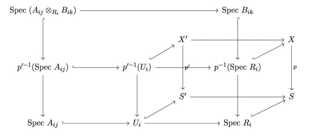
is of finite type, giving us the desired cover of  . The following diagram may be illustrative (every square is a pullback)
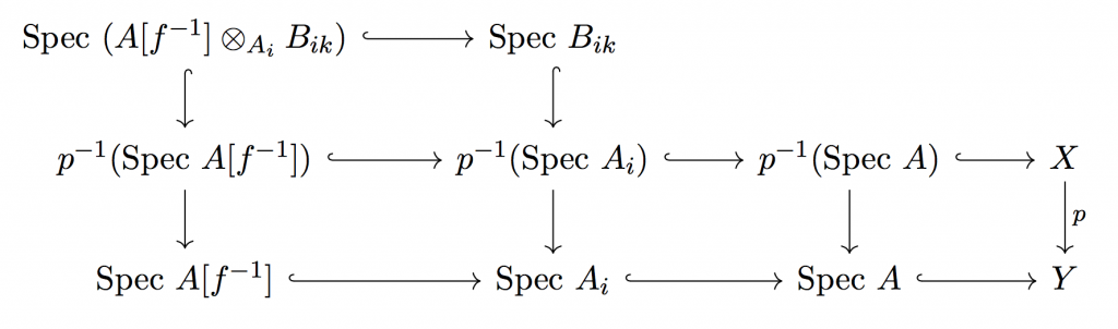
 on
on  defines a
  -grading of
  . A future post may describe how this relates to projective schemes. (I will do all of this using diagrams, but there may be some easier way using the functors of points). All this was taught to me by Mark Haiman in Math 256B (Algebraic Geometry) at UC Berkeley.
 ; we will work in the category of
  , rather than selecting some point in the underlying topological space.
![\text{Spec }k[s, t]/(st-1) = \text{Spec }k[t, t^{-1}]](https://www.ocf.berkeley.edu/~rohanjoshi/wp-content/ql-cache/quicklatex.com-14d0a07c6c7d1e492a76a6f14e61260e_l3.png "Rendered by QuickLaTeX.com") . (for shorthand, we will write
. (for shorthand, we will write ![k[t, t^{-1}]](https://www.ocf.berkeley.edu/~rohanjoshi/wp-content/ql-cache/quicklatex.com-ef4cf6391ea8b37b14e0110a429d4e24_l3.png "Rendered by QuickLaTeX.com") as
as ![k[t^\pm]](https://www.ocf.berkeley.edu/~rohanjoshi/wp-content/ql-cache/quicklatex.com-1a3c5786109dabd7b13fd9dda9a54987_l3.png "Rendered by QuickLaTeX.com") ). As a variety, it can be thought of as
). As a variety, it can be thought of as  , the “punctured affine line”. Its group operation is given by a map
  which corresponds to the
 ![\mu: k[t^\pm] \to k[t^\pm] \otimes_k k[t^\pm] \cong k[t^\pm, u^\pm]](https://www.ocf.berkeley.edu/~rohanjoshi/wp-content/ql-cache/quicklatex.com-79f03678c9d18a031f3fea81f7fc8169_l3.png "Rendered by QuickLaTeX.com") defined by
defined by  . The identity is given by a map
  corresponding to
 ![i: k[t^\pm] \to k](https://www.ocf.berkeley.edu/~rohanjoshi/wp-content/ql-cache/quicklatex.com-62ac99a2afee5ef00ba206cc512831fd_l3.png "Rendered by QuickLaTeX.com") defined by
defined by  .
. . The action map
  corresponds to a
 ![\phi: R \to R \otimes_k k[t^\pm] \cong R[t^\pm]](https://www.ocf.berkeley.edu/~rohanjoshi/wp-content/ql-cache/quicklatex.com-aa15fc6f0c24ec4637214cc05d08c13e_l3.png "Rendered by QuickLaTeX.com") such that the following diagrams commute:
such that the following diagrams commute:![\xymatrix{R\ar[r]^{\phi}\ar[d]^{\phi} & {R[t^\pm]} \ar[d]^{id_R\otimes \mu}\\{R[u^\pm]} \ar[r]^{\phi \otimes id_{k[u^\pm]}} & {R[t^\pm, u^\pm]}}](https://www.ocf.berkeley.edu/~rohanjoshi/wp-content/ql-cache/quicklatex.com-be58b01614e66fda49f67e15ebbc62ce_l3.png "Rendered by QuickLaTeX.com")
![\xymatrix{R\ar[r]^{\phi}\ar[d]^{id_R} & {R[t^\pm]} \ar[dl]^{i}\\ R}](https://www.ocf.berkeley.edu/~rohanjoshi/wp-content/ql-cache/quicklatex.com-328480c25d8ee63a186221bdc075521c_l3.png "Rendered by QuickLaTeX.com")
 , write
 ![\phi(r) = \sum_{-\infty}^{\infty} r_it^i \in R[t^\pm]](https://www.ocf.berkeley.edu/~rohanjoshi/wp-content/ql-cache/quicklatex.com-68f8bcaece4bbfb72383434b60314468_l3.png "Rendered by QuickLaTeX.com") , where almost all the
, where almost all the  are zero. Then the first diagram implies that
  (i.e. the polynomial is just a single monomial), then
  .
. and along the left and bottom arrows we have
  . Furthermore, the second diagram says that
  for all
  ,
,  .
.![R[t^\pm]_d](https://www.ocf.berkeley.edu/~rohanjoshi/wp-content/ql-cache/quicklatex.com-55044f31798484cbc940a50a3ddb2c0d_l3.png "Rendered by QuickLaTeX.com") stand for the degree
stand for the degree  homogenous component of
 ![R[t^\pm]](https://www.ocf.berkeley.edu/~rohanjoshi/wp-content/ql-cache/quicklatex.com-ec8240204187e3417fd0eb6ee424892f_l3.png "Rendered by QuickLaTeX.com") (so that it consists of multiples of
(so that it consists of multiples of  ), let
 ![R_d := \phi^{-1}(R[t^\pm]_d)](https://www.ocf.berkeley.edu/~rohanjoshi/wp-content/ql-cache/quicklatex.com-65279920cb1f39bc1f761221fba04b07_l3.png "Rendered by QuickLaTeX.com") . Since all the
. Since all the  by
by  . Thus
  as a direct sum.
 . But this is easy: if
  , then
 ![\phi(r_mr_n) = \phi(r_m)\phi(r_n) = r_mr_nx^{m+n} \in R[t^\pm]_{m+n}](https://www.ocf.berkeley.edu/~rohanjoshi/wp-content/ql-cache/quicklatex.com-101cef2c6151d2acad5c8e06940b0acb_l3.png "Rendered by QuickLaTeX.com") , so
, so  as desired.