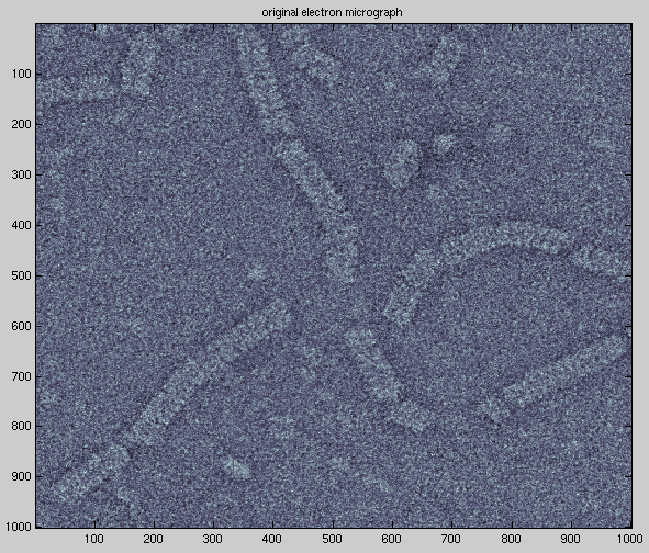
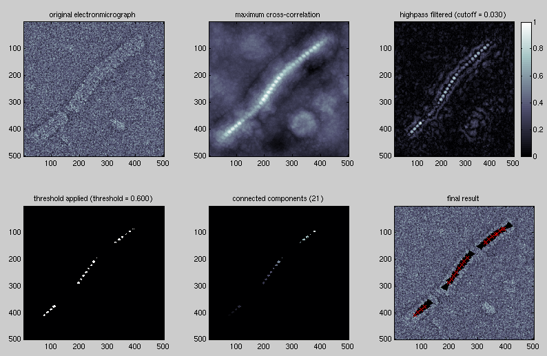
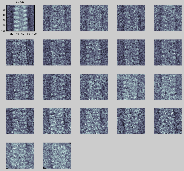
The process starts with an electron micrograph containing particles that we'd like to locate. In this case the "particles" are helical structures, which are conveniently lying flat in the horizontal plane. We already have a reference projection of a small segment of helix, and this is the pattern for which we will search.
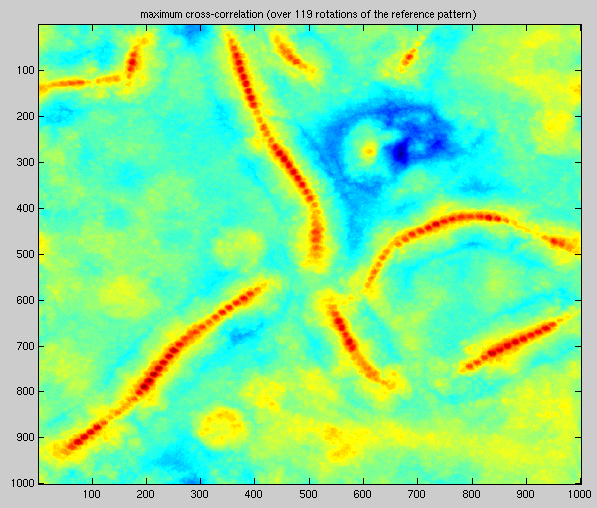
To find the reference pattern in the electron micrograph, we form the cross-correlation of the micrograph and the reference pattern. Since the pattern may be rotated in the plane, we form the cross-correlation of the micrograph with a series of rotations of the reference pattern. The resulting image (below) is formed by taking the maximum on a pixel-by-pixel basis of this collection of cross-correlations. (See pattern matching by cross correlation.)
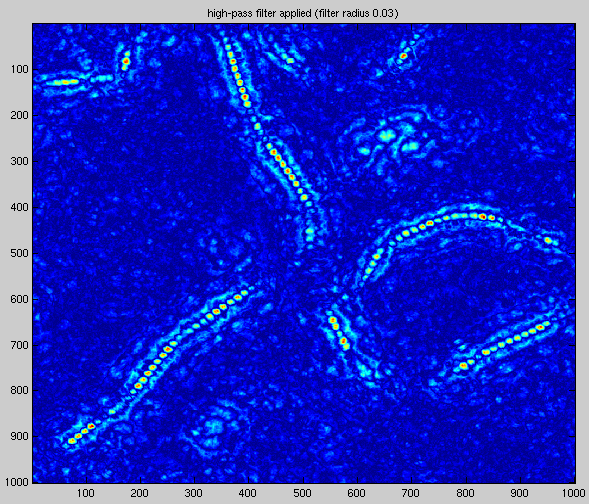
We need to find the peaks in the above image, and to do this we first make them more distinct by applying a high-pass filter. This eliminates the broad plateus and other high-valued areas that might confuse our peak-finding algorithm. In the resulting image the peaks corresponding to particle matches are quite distinct:
Now a threshold is applied to the image. The image is first normalized so that pixel values may range from 0 to 1. Then pixels with value higher than 0.6 are set to 1, and the remainder are set to zero. A cluster identification algorithm is then applied to locate the connected components of the image.
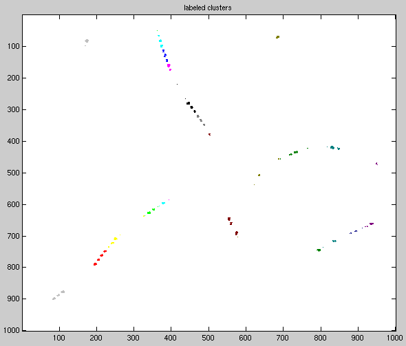
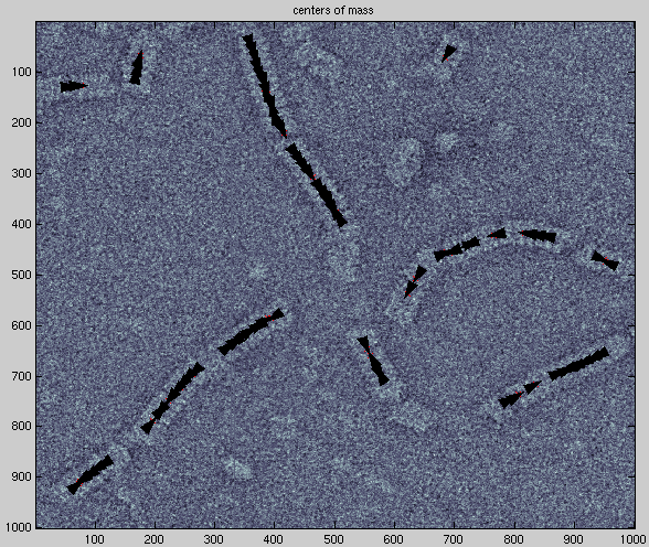
Each cluster in the above image is composed of a small number of pixels grouped together. We can compute a "center of mass" for each cluster by considering each pixels "mass" to be its intensity in the cross-correlation plot. For each pixel we multiply the pixel's coordinates by its mass, and divide by the total mass of the cluster; add up all these values for each cluster and we get the center of mass.
Not only do we now have positions for each particle detection, but we also have the orientation angle for each particle detection as well, since we can look these up from the original correlation data (when we found the maximum of the correlations for each orientation, we also recorded the angle that resulted in that best correlation). So, for our final results, we can draw not only an "x" at the detection location, but an arrow indicating the detected particle orientation:
Finally, here's an overview of the whole process:
Go up